List the postulates of kinetic theory of gases. Derive one kinetic gas equation?
1 Answer

The main postulates or assumptions are (for ideal gases):
- Gases are constantly in motion, colliding elastically in their container.
- They do not interact (i.e. no intermolecular forces are considered), and are assumed to be point masses with negligible volume compared to the size of their container.
- Ensembles of gases produce a distribution of speeds, and the average kinetic energy of this ensemble is proportional to the translational kinetic energy of the sample.
As for "one kinetic gas equation", there is not just one. But I can derive the Maxwell-Boltzmann distribution, and from there one could derive many other equations... some of them being:
- collision frequency
- average speed
- RMS speed
- most probable speed
The latter three are derived in more detail here.
The following derivation is adapted from Statistical Mechanics by Norman Davidson (1969). Fairly old, but I kinda like it.
Consider the classical Hamiltonian for the free particle in three dimensions:
#H = (p_x^2)/(2m) + (p_y^2)/(2m) + (p_z^2)/(2m)# ,where
#p = mv# is the momentum and#m# is the mass of the particle.
The distribution function will be denoted as
From Statistical Mechanics by Norman Davidson (pg. 150), we have that
#(dN)/N = (e^(-betaH(p_1, . . . , p_n; q_1, . . . , q_n)) dp_1 cdots dp_n dq_1 cdots dq_n)/zeta# ,where:
#beta = 1//k_BT# is a constant, with#k_B# as the Boltzmann constant and#T# as the temperature in#"K"# .#H(p_1, . . . , p_n; q_1, . . . , q_n)# is the Hamiltonian for a system with#3N# momentum coordinates and#3N# position coordinates, containing#N# particles in 3 dimensions.#zeta = int cdots int e^(-betaH(p_1, . . . , p_n; q_1, . . . , q_n)) dp_1 cdots dp_n dq_1 cdots dq_n# is the classical phase integral.
This seems like a lot, but fortunately we can look at three coordinates for simplicity.
A phase integral is an integral over
With
#(dN(p_x,p_y,p_z; x,y,z))/(N) = ("exp"(-(p_x^2 + p_x^2 + p_z^2)/(2mk_BT))dp_xdp_ydp_z)/(int_(-oo)^(oo) int_(-oo)^(oo) int_(-oo)^(oo) "exp"(-(p_x^2 + p_x^2 + p_z^2)/(2mk_BT))dp_xdp_ydp_z)#
Now, let's take the bottom integral and separate it out:
#zeta = int_(-oo)^(oo) e^(-p_x^2//2mk_BT)dp_x cdot int_(-oo)^(oo) e^(-p_y^2//2mk_BT)dp_y cdot int_(-oo)^(oo) e^(-p_z^2//2mk_BT)dp_z#
In phase space, each of these integrals are identical, except for the particular notation. These all are of this form, which is tabulated:
#2int_(0)^(oo) e^(-alphax^2)dx = cancel(2 cdot 1/2) (pi/alpha)^(1//2)#
Notice how the answer has no
#zeta = (2pimk_BT)^(3//2)#
So far, we then have:
#(dN(p_x,p_y,p_z; x,y,z))/(N) = ("exp"(-(p_x^2 + p_x^2 + p_z^2)/(2mk_BT))dp_xdp_ydp_z)/(2pimk_BT)^(3//2)#
Next, it is convenient to transform into velocity coordinates, so let
#(dN(v_x,v_y,v_z; x,y,z))/(N) = (e^(-m^2(v_x^2 + v_y^2 + v_z^2)//2mk_BT)m^3dv_xdv_ydv_z)/(2pimk_BT)^(3//2)#
#= (m/(2pik_BT))^(3//2)e^(-m(v_x^2 + v_x^2 + v_z^2)//2k_BT)dv_xdv_ydv_z#
Now, we assume that the gases are isotropic, meaning that no direction is any different from any other.
To enforce that, suppose we enter velocity space, a coordinate system analogous to spherical coordinates, but with components of
#v_x = vsintheta_vcosphi_v#
#v_y = vsintheta_vsinphi_v#
#v_z = vcostheta_v#
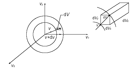
With the differential volume element being
#(dN(v, theta_v, phi_v))/(N)#
#= (m/(2pik_BT))^(3//2) cdot e^(-m(v^2sin^2theta_v cos^2phi_v + v^2 sin^2theta_v sin^2phi_v + v^2 cos^2theta_v)//2k_BT)v^2 dv sintheta_v d theta_v d phi_v#
Fortunately, using
#= (m/(2pik_BT))^(3//2) cdot e^(-m(v^2sin^2theta_v(cos^2phi_v + sin^2phi_v) + v^2 cos^2theta_v)//2k_BT)v^2 dv sintheta_v d theta_v d phi_v#
#= (m/(2pik_BT))^(3//2) cdot e^(-m(v^2sin^2theta_v + v^2 cos^2theta_v)//2k_BT)v^2 dv sintheta_v d theta_v d phi_v#
#=> ul((dN(v, theta_v, phi_v))/(N) = (m/(2pik_BT))^(3//2)e^(-mv^2//2k_BT)v^2 dv sintheta_v d theta_v d phi_v)#
We're almost there! Now, the integral over allspace for
#int_(0)^(pi) sintheta_vd theta_v = 2#
And the integral over allspace for
#int_(0)^(2pi) dphi_v = 2pi#
So, we integrate both sides to get:
#color(blue)(barul(|stackrel(" ")(" "(dN(v))/(N) -= f(v)dv = 4pi (m/(2pik_BT))^(3//2)e^(-mv^2//2k_BT)v^2 dv" ")|))#
And this is the Maxwell-Boltzmann distribution, the one you see here:

DERIVATION OF SOME OTHER EQUATIONS
This is only a summary.
Gas Speed Equations
#<< v >> = int_(0)^(oo) vf(v)dv = sqrt((8k_BT)/(pim)#
#v_(RMS) = << v^2 >>^(1//2) = (int_(0)^(oo) v^2f(v)dv)^(1//2) = sqrt((3k_BT)/m)#
#v_(mp)# : Take the derivative of#f(v)# , set the result equal to#0# , and solve for#v# to get
#v_(mp) = sqrt((2k_BT)/m)#
