Without going too far into the details of probability theory, "P"(* )P(⋅) is like a function that takes in events, or subsets of a sample space, and maps them to numbers between 0 and 1 (similar to how f(*)f(⋅) might be a function that takes in real numbers and maps them to other real numbers).
Quick example: let EE be the event that a single coin toss lands heads-up. Then the probability of EE occurring is one-half:
Sample space S={"H","T"}S={H,T}
Subset E={"H"}E={H}
"P"(E)=("size of "E)/("size of "S)=1/2.P(E)=size of Esize of S=12.
Elements of a sample space can be encoded into random variables. To do this, we just map each element of the sample space to a number. In the coin toss example, we could map "heads" to 11, and "tails" to 00. We also need a variable that could take on these number values; a common choice is XX. So we could rewrite "P"(E)=1/2P(E)=12 using the random variable XX, like this:
"P"(X=1)=1/2.P(X=1)=12.
The probability of "event EE occurring" is the same as the probability of "XX being equal to 1".
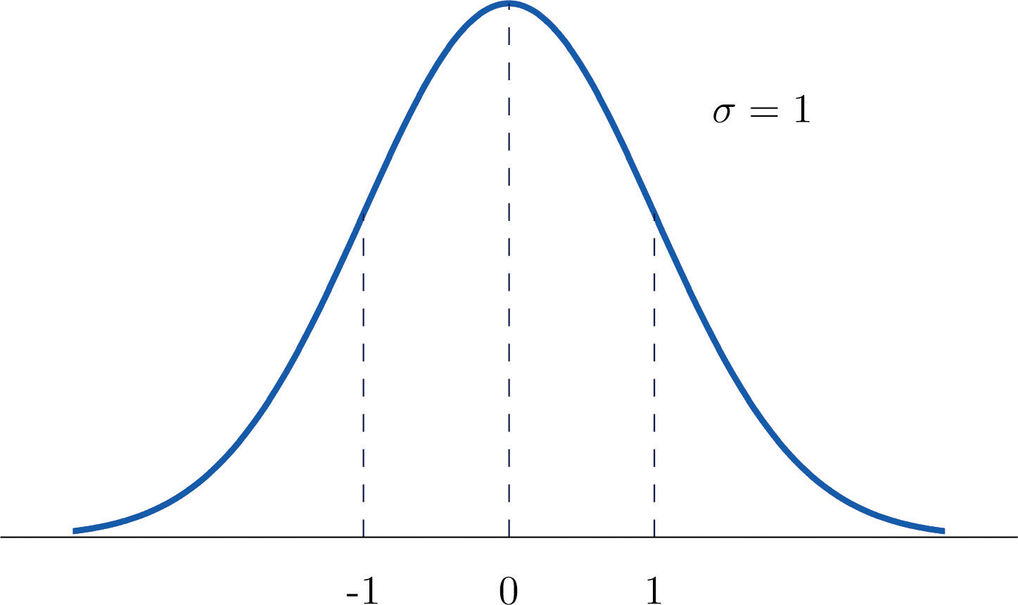
Skipping a few chapters in statistics, there are many special types of random variables that have useful distributions, or patterns in how they map events to numbers. One such common random variable is called ZZ, and it follows the standard normal distribution. Ever hear of a bell curve? Well, ZZ is the most basic of all bell curves. The peak of ZZ's curve is at 0, and the variance (or "spread") of the curve is 1:
 saylordotorg.github.io
ZZ is so useful because we can "translate" any other normal random variable into ZZ by shifting it left/right by its mean, and then squishing/stretching it by its standard deviation. In math terms, for any normal random variable XX with mean muμ and standard deviation sigmaσ, we have
"P"(X < x)="P"(Z<(x-mu)/sigma)P(X<x)=P(Z<x−μσ)
That's why we have zz-tables. We don't need a "normal table" for every normal distribution XX because we can just map the points in the XX distribution to equivalent points in the ZZ distribution.
Alright, enough background. You need to know how to find "P"(Z<1.37)P(Z<1.37). This is the area under the ZZ curve between -oo−∞ and 1.371.37. A zz-table lets you look up a zz-value (like z=1.37z=1.37) and shows you a matching probability, but there are two ways a table may choose to do this. It may show you:
- the probability of ZZ being less than zz (lower-tail)
- the probability of ZZ being greater than zz (upper-tail)
It is up to you to know how to interpret the matching probability for your zz-value. If the probabilities get closer to 1 as zz goes up, then your table shows "P"(Z < z)P(Z<z) (known as the cumulative probability). If the probabilities get closer to 0 as zz goes up, then your table is showing you P(Z > z)P(Z>z). Fortunately, we can work with both.
If we want P(Z < z)P(Z<z), and our table gives us P(Z>z),P(Z>z), we just need to use the fact that the total area under any random variable's distribution curve is always 1. Meaning:
"P"(Z < z)" "+" ""P"(Z > z)" "=" "1P(Z<z) + P(Z>z) = 1
or
"P"(Z < z)" "=" "1" "-" ""P"(Z > z)P(Z<z) = 1 − P(Z>z)
So for example, if you look up z=1.37z=1.37 in your table, and it gives you an upper-tail area of 0.0853, you know the area to the left of that zz-value must be 0.9147, since 0.0853+0.9147=1.0.0853+0.9147=1.