Calculate the limiting value of the fraction of dissociation (α) of a weak acid (pKa = 5.00) as the concentration of HA approaches 0. Repeat the same calculation for pKa = 9.00.?
2 Answers

Explanation:
Let's first calculate the expression for α for a weak acid
color(blue)(bar(ul(|color(white)(a/a)α =("-"K_text(a) + sqrt(K_text(a)^2 + 4K_text(a)c))/(2c)color(white)(a/a)|)))" "
Fortunately, "they" didn't specify how we were to calculate the limit.
I chose to calculate the limit by inserting progressively smaller values for the molar concentration
I used Microsoft Excel to calculate the values of α for concentrations ranging from
I got the following table:
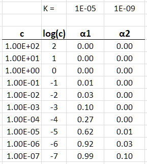 Table
Table
Normally, we will not encounter solutions as concentrated as
Next, I plotted
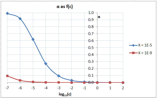 Graph
Graph
The graph shows that a weak acid like acetic acid is almost completely dissociated when
That is,
However, an even weaker acid like

The fraction of dissociation
The only thing that changes with a smaller
All that matters for convergence of
First, let's consider what fraction of dissociation means.
alpha = (["HA"]_"lost")/(["HA"]_i)
The
alpha = (["H"^(+)])/(["HA"]_i) -= x/(["HA"]_i)
bb(lim_(["A"]_i -> 0) alpha = 1) .
The condition, as shown in this video, is that
K_a/(["HA"]_i) < 1
for the small
What I shall do is decrease
At each iteration up until the final one, we have:
x_1 ~~ sqrt(["HA"]_i cdot K_a)
x_2 ~~ sqrt((["HA"]_i - x_1)cdot K_a)
x_3 ~~ sqrt((["HA"]_i - x_2)cdot K_a)
vdots
x_N ~~ sqrt((["HA"]_i - x_(N-1))cdot K_a)
With that in mind, I did this in Excel just now, supposing that
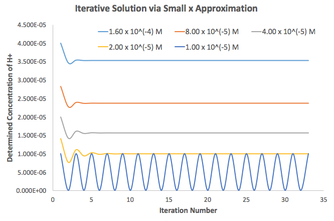
The data graphed was:
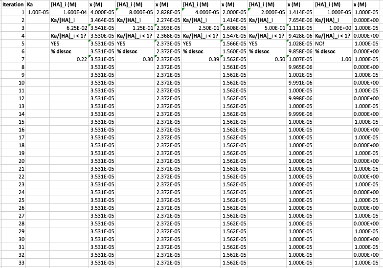
Things to scan for on the data:
-
Decreasing concentrations
["HA"]_i were used, starting from["HA"]_i = K_a and doubling from right to left. -
As
["HA"]_i decreases, more iterations are required for convergence. When["HA"]_i gets too small (smaller thanK_a ), convergence is impossible (see the sine wave?). -
There was an if conditional, i.e.
"If K"_a//["HA"]_i < 1 , then say"YES" .
"Else" , say"NO!" I was showing here then, that if
K_a//["HA"]_i >= 1 , the smallx approximation fails catastrophically.
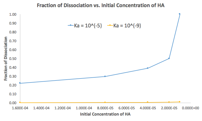
- I calculated the
%"dissoc" , which was0.22, 0.30, 0.39, 0.50, 1.00 , i.e. it approachesbb1 as["HA"]_i decreases. It is1 whenK_a = ["HA"]_i .
We can now see the issue: since
- If we have the
(n-1) th value,x_(n-1) , less than["HA"]_i , thenx_n converges monotonically. - If we have the
(n-1) th value,x_(n-1) , equal to["HA"]_i , thenx_n oscillates between0 andK_a . - If we have the
(n-1) th value,x_(n-1) , greater than["HA"]_i , thenx_n is imaginary.
I did the same thing for
So now, let's consider
This graph is then:
And here we do see that
