Question

How to calculate the exponents in the differential rate law?

GIVEN:

Answer 1

You use the formulas from the integrated rate laws.

Explanation:

Shen you have a list of concentrations as a function of time, you want to plot something that gives a straight line.

The equation for a straight line is:

`color(blue)(bar(ul(|color(white)(a/a) y = mx + b color(white)(a/a)|)))" "`

We can write the integrated rate laws for zero-, first, and second-order reactions all as straight-line functions.

`ulbb("Order"color(white)(mll)y = color(white)(l)mcolor(white)(l)x + b)`
`color(white)(mll)0 color(white)(mmml)c = color(white)(l)"-"kcolor(white)(ll)t + c_0`
`color(white)(mll)1color(white)(mm)lnc = color(white)(l)"-"kcolor(white)(ll)t + lnc_0`
#color(white)(mll)2color(white)(mmm)1/c = color(white)(ll )kcolor(white)(ll)t + 1/c_0#

Thus,

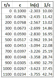
• For a 0-order reaction, a plot of `c` vs `t` should give a straight line with slope `"-"k`
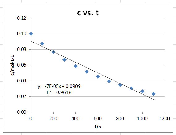
• For a 1st-order reaction, a plot of `ln(c)` vs `t` should give a straight line with
  slope `"-"k`
• For a 2nd-order reaction, a plot of `1/c` vs `t` should give a straight line with slope `k`

So, we plot each of these functions and see which gives the best straight line.

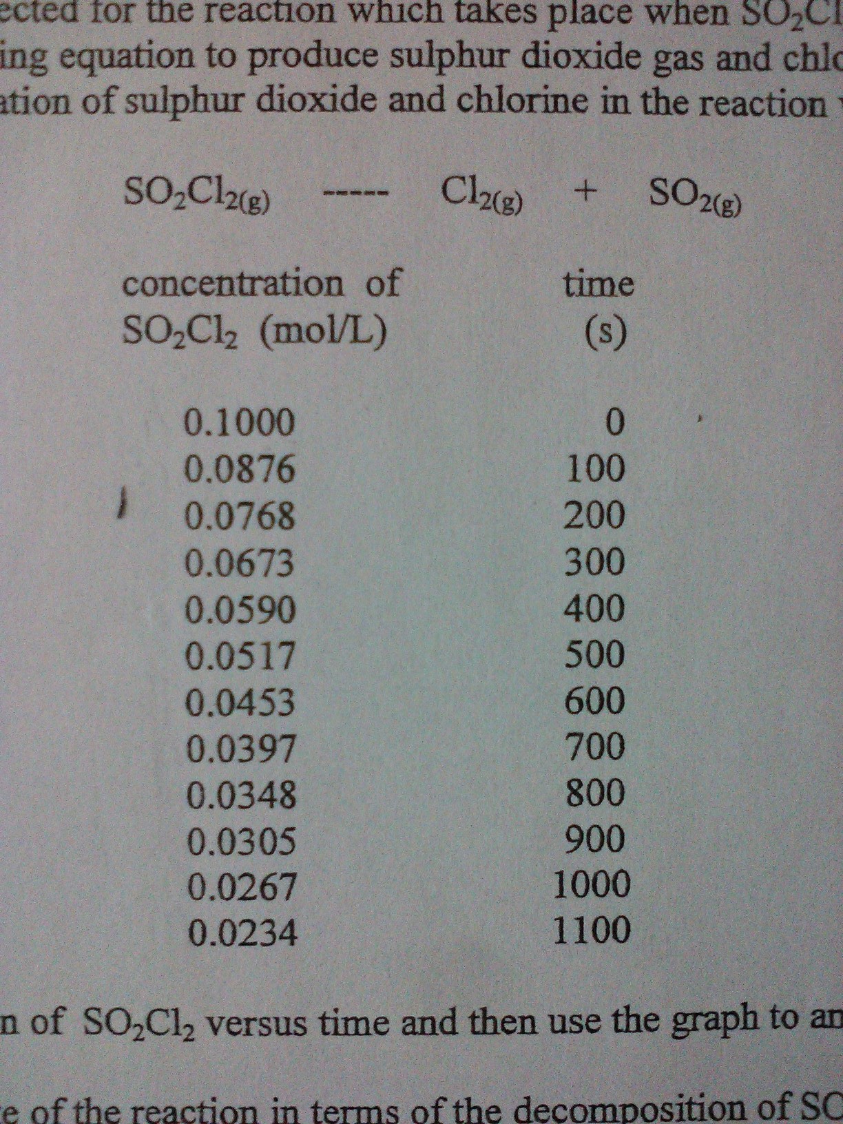
I used Excel to convert your data into the following table.

Then I plotted each of the three functions.

Zero-Order Plot

The graph appears to be a curve.

First-Order Plot

The graph appears to be a straight line.

Second-Order Plot

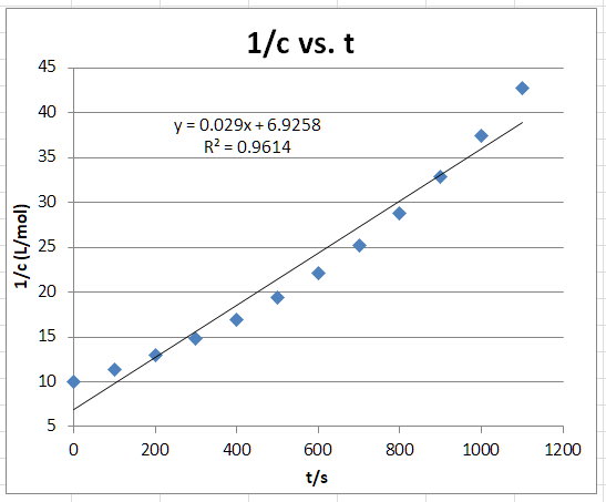
The graph appears to be a curve.

Conclusion

Your data give the best fit to a first-order rate law of the form

`rate = k["SO"_2"Cl"_2]^1`

Answer 2

Jose suggested a different way to approach this, so I figured I'd share it.

---

The starting rate law is:

`r(t) = k["SO"_2"Cl"_2]^m`

Jose suggested that one could take the `ln` of both sides like this:

`ln r(t) = mln["SO"_2"Cl"_2] + lnk`

But this requires that we generate a new column of data:

`r(t) = -(Delta["SO"_2"Cl"_2])/(Deltat)`

and for `n` data points, we generate `n-1` new data points to use here. We use the midpoint concentrations of `"SO"_2"Cl"_2` (call them `["SO"_2"Cl"_2]_"mp"`) and generate each `r(t)` as described above.

`ul(ln[r(t) xx 10^4] ("M/s")" "" "" "ln["SO"_2"Cl"_2]_"mp" ("M")" ")`

`ln1.24" "" "" "" "" "" "" "" "" "ln0.0938`
`ln1.08" "" "" "" "" "" "" "" "" "ln0.0822`
`ln0.95" "" "" "" "" "" "" "" "" "ln0.0721`
`ln0.83" "" "" "" "" "" "" "" "" "ln0.0632`
`ln0.73" "" "" "" "" "" "" "" "" "ln0.0554`
`ln0.64" "" "" "" "" "" "" "" "" "ln0.0485`

You get the idea. I'll leave out the remaining `5` data points because six is quite sufficient to establish a trend.

Plotting `lnr(t)` vs. `ln["SO"_2"Cl"_2]`, the y-intercept should be `lnk`, and the slope should be whatever the order of reaction is.

The regression equation was found as follows using my trusty TI-83 calculator.

1. `"STAT"` `->` `"Edit"`, enter all the data in there. Have the `x` variable in `"L1"` and `y` variable in `"L2"`.
2. `"STAT" -> "CALC" -> "LinReg"("ax+b")`

This gave:

`lnr(t) = 1.000765854 cdot ln["SO"_2"Cl"_2]_"mp" - 6.630082087`

This implies that the order of reaction is approx. `color(blue)(1)` and that

`lnk = -6.630082087`

and

`color(blue)(k) = e^(-6.630082087) = color(blue)("0.0013 s"^(-1))`

So this method works too. However, you can see it is a big hassle, when you have this many data points, to rewrite all of them into `lnr(t)` and `ln["SO"_2"Cl"_2]_"mp"`. I would say Ernest's method is faster.