Question

Question about contingency table?

How to construct a contingency table between two variables and show whether there is a relationship between the two variables at α = 5% significance level?

Answer 1

A contingency table is a two-way table whose cells contain the observed values of a dependent random variable under all different combinations of two other random variables.

Suppose we are asking a group of 115 people what their favourite game and snack is (from the given options). After the data are collected, the contingency table might look like this:

For instance, the cell in row "Monopoly" and column "Chips and Dip" says we observed 17 people who said both Monopoly is their favourite game and chips & dip is their favourite snack.

To test if there is a relationship between the "Game" and "Snack" variables, we need to see if the observed values are different enough from what we would expect if they were not related.

Sample calculation, expected value of cell (1,1): if there were no relation between "Game" and "Snack", then we would expect the fraction of poker players that also like pizza rolls to match the fraction of everybody that likes pizza rolls. Mathematically, this is written as

`E_11/y_(1*)=y_(*1)/y_(* *)`

where

`E_11` is the expected value for cell (1,1),
`y_(1*)` is the total for row 1 (25),
`y_(*1)` is the total for column 1 (44), and
`y_(* *)` is the grand total (115).

Then we solve for `E_11:`

`E_11/25 = 44/115`

`E_11 = 25*44/115" " ~~ 9.565`

This is repeated for all cells.

Once you have the expected values, you see how big all the (squared) differences between each observed value to its expected value are, compared to just their expected values. This is known as a chi-squared `(chi^2)` statistic, and its formula (for a contingency table) is:

`c^2 = sum_(i,j)[(O_(ij)-E_(ij))^2/E_(ij)]`

The idea is that, if the observed values are not that different from the expected values, the numerators will be small compared to the denominators, and so the sum of all these fractions `(c^2)` will be small too. But if `c^2` is too high, then the observations are too different from their expected values, and we conclude there is significant evidence of a relation.

Sample calculation, `chi^2` element (1,1):

`(O_(11)-E_(11))^2/E_(11)=(10-9.565)^2/(9.565)=0.020`

Again, this is repeated for all cells; the sum of all these values will be `c^2`.

After summing all the ratios of `(O-E)^2/E`, you'll get `c^2 = 14.508.` Now we ask: is this big or not? We need a number to compare this to. That will be the value `chi_(1-alpha, (n-1)(k-1))^2,` which is the coordinate of the `chi^2` distribution with `(n-1)(k-1)` degrees of freedom that has `100(1-alpha)%` of the area to its left. (`n` and `k` are the number of rows and columns in our table.)

Why use `chi^2`? Because we assume each `O_(ij)` is Normal, and so `[O_(ij)-E_(ij)]/sqrt(E_(ij))` is Standard Normal, and the sum of a bunch of squared Standard Normal random variables has a `chi^2` distribution.

Using a table (or software), we look up `chi_(0.95, 6)^2 = 12.592`. Since our value of `c^2 = 14.508` is larger than `chi_(0.95, 6)^2 = 12.592`, we conclude that `c^2` is too large to have come from a `chi^2` distribution (with 6 d.f.) and that there is a relation between "Game" and "Snack" (at significance level `alpha = 0.05`).

Answer 2

Refer explanation section

Explanation:

A contingency table is formed to show two attributes of a same phenomenon say a person.
In this Table, one attribute is favourite snacks. It is shown along the column. Another attribute is favourite game. It is shown along the row. We collected data from 115 Persons. We tabulated the data.

How to interpret the table? Take first row first column (R1C1) ; It shows 10 persons who are fond of Poker games are mad after the snack. This is how you have to interpret all the cells.

The purpose of forming the table is to find – is there any relation between two attributes. We conduct a test. The name of the test is chi-square test. We form null hypothesis
Ho : Preference of snack is independent of preference for game.
Our conclusion, if the test result shows otherwise is shown in the form of alternate hypothesis.

H1: Preference of snack depends of preference for game.

How to Organise the test? What is given in the table is observed frequency. For each cell we have to calculate expected frequency. It is given in the following table.

Find (0-E)^2/E for each cell. The sum of this is calculated chi-square value. It is 14.5. We have to compare with the table chi-square value. Refer the table for 5% significance and 6 degrees of freedom. It is 12.6.

Look at the graph-

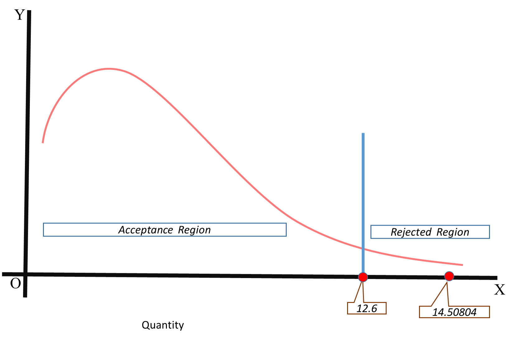
The calculated chi-square value is higher than the table chi-square value. The calculated chi-square value lies in the rejected region. So, null hypothesis is rejected. Alternate hypothesis is accepted. It means, the preference for snacks very much depends on the type of game an individual play.