Question

Titration curve? Please help...

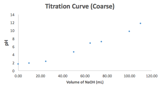
50ml of 0.100M H3PO4 is titrated with 0.100M NaOH (i) calculate the pH after the addtion of the following volumes of titrant; 0.00, 10.00, 25.00, 50.00, 65.00, 75.00, 100.00, and 110.00. Note that since Ka1 is relatively large, the complete quadratic should be solved for the first three volumes. (ii) Plot the titration curve.
answers (i) 1.62; 1.89; 2.26; 4.67; 6.84; 7.21; 9.77; 11.72; (ii) Graph

Answer 1

Well, first I would sketch the titration curve of a diprotic acid (`"HPO"_4^(2-)` is hard enough to form).

Here we distinguish between the buffer region (wherein the half-equivalence point lies) and the equivalence point.

• Buffer region --- Henderson-Hasselbalch equation does NOT apply UNLESS the current `K_a` is small. `K_(a1)` is not small enough, but `K_(a2)` and `K_(a3)` are.
• Half-equivalence point --- `"pH" = "pK"_a`
• Equivalence point --- Regular weak acid/base equilibrium!

`K_(a1,2,3) = 7.1 xx 10^(-3), 6.3 xx 10^(-8), 4.5 xx 10^(-13)`

So we first find the equivalence points.

`"H"_3"PO"_4 + 3"NaOH"(aq) -> "Na"_3"PO"_4(aq) + 3"H"_2"O"(l)`

`"Total equivalence point"`:

`"0.100 mol"/"L" xx "0.050 L" = "0.0050 mols H"_3"PO"_4`

`= "0.0150 mols OH"^(-)`

`=> "1000 mL"/"0.100 mol NaOH" xx "0.0150 mols OH"^(-)`

`=` `"150 mL"` for all three protons

`=>` `"50 mL"` for each proton

Thus, the equivalence points are at `"50 mL"`, `"100 mL"`, and `"150 mL"`. Notice how we don't reach `"150 mL"`, so ignore that one.

`(ia)` `"0.00 mL"` base added

`"H"_3"PO"_4(aq) rightleftharpoons "H"_2"PO"_4^(-)(aq) + "H"^(+)(aq)`

`K_(a1) = 7.1 xx 10^(-3) = (["H"_2"PO"_4^(-)]["H"^(+)])/(["H"_3"PO"_4]) = x^2/(0.100 - x)`

Although `x` is not small enough, since `(K_(a1))/("0.100 M") < 1`, this can be done iteratively.

`x_1 ~~ sqrt(0.100K_(a1)) = "0.02665 M"`

`x_2 ~~ sqrt((0.100 - x_1)K_(a1)) = "0.02282 M"`

`x_3 ~~ sqrt((0.100 - x_2)K_(a1)) = "0.02341 M"`

`x_4 ~~ sqrt((0.100 - x_3)K_(a1)) = "0.02332 M"`

`x_5 = sqrt((0.100 - x_4)K_(a1)) = "0.02333 M"`

And thus, `x = "0.02333 M"` for `["H"^(+)]`. That gives

`color(blue)("pH"_1) = -log(0.02333) = color(blue)(1.63)`.

`(ib)` `"10.00 mL"` of base added

`"0.100 mol/L" xx "0.010 L" = "0.0010 mols OH"^(-)`

This neutralizes that much `"H"_3"PO"_4` to give

`"0.0050 mols H"_3"PO"_4 - "0.0010 mols OH"^(-)`

`= "0.0040 mols H"_3"PO"_4` leftover

`-> "0.0010 mols H"_2"PO"_4^(-)` produced

This is then a concentration of

`("0.0010 mols H"_2"PO"_4^(-))/("50.00 mL acid" + "10.00 mL base") cdot "1000 mL"/"1 L"`

`=` `"0.01667 M H"_2"PO"_4^(-)`

and `"0.06667 M H"_3"PO"_4`

These again go into the full equilibrium expression. Remember to include the initial concentrations.

`K_(a1) = 7.1 xx 10^(-3) = (["H"_2"PO"_4^(-)]["H"^(+)])/(["H"_3"PO"_4])`

`= ((0.01667 + x)(x))/(0.06667 - x)`

This must be solved in full.

`7.1 xx 10^(-3) cdot 0.06667 - 7.1 xx 10^(-3)x = 0.01667x + x^2`

`x^2 + (0.01667 + 7.1 xx 10^(-3))x - 7.1 xx 10^(-3) cdot 0.06667 = 0`

`x^2 + 0.02377x - 4.73 xx 10^(-4) = 0`

and here we get `["H"^(+)] = x = "0.01290 M"`, so

`color(blue)("pH"_2) = -log(0.01290) = color(blue)(1.89)`

`(ic)` `"25.00 mL"` of base added, the first half-equivalence point

I won't show much math here, but you can convince yourself that you are at the first half-equivalence point, so

`"pH"_3 = "pK"_(a1) = -log(7.1 xx 10^(-3)) ~~ 2.15` is expected.

However, it's a bit larger, due to Le Chatelier's principle.

`["H"_2"PO"_4^(-)] = ["H"_3"PO"_4] = "0.0025 mols"/("50.00 mL acid" + "25.00 mL base") cdot "1000 mL"/"1 L"`

`=` `"0.03333 M"`

`K_(a1) = 7.1 xx 10^(-3) = (["H"_2"PO"_4^(-)]["H"^(+)])/(["H"_3"PO"_4])`

`= ((0.03333 + x)(x))/(0.03333 - x)`

Solving this, we find

`0 = x^2 + (0.03333 + 7.1 xx 10^(-3))x - 7.1 xx 10^(-3) cdot 0.03333`

for which `x = ["H"^(+)] = "0.005188 M"` and

`color(blue)("pH"_3) = -log(0.005188) = color(blue)(2.29)`

`(id)` `"50.00 mL"` of base added, the first equivalence point

Here we are halfway between the first and second half-equivalence points, which had `"pH" = "pK"_(ai)`, so

`color(blue)("pH"_4 = 1/2("pK"_(a1) + "pK"_(a2)) = 4.67)`

`(ie)` `"65.00 mL"` of base added, or `"15.00 mL"` past first equivalence point

`"0.0015 mols NaOH"` added to neutralize `"0.0015 mols H"_2"PO"_4^(-)` to give `"0.0015 mols HPO"_4^(2-)` and `"0.0035 mols H"_2"PO"_4^(-)` in `"50.00 + 65.00 mL"` solution.

The Henderson-Hasselbalch equation here would apply, since `K_(a2)` is small. The `K_(a2)` would be:

`6.3 xx 10^(-8) = ((0.01304 + x)(x))/(0.03043 - x) ~~ (0.01304x)/0.03043`

`=> x ~~ 1.470 xx 10^(-7) "M"`

and `color(blue)("pH"_5 ~~ 6.83)`.

Or, we could have done...

`"pH"_5 = "pK"_(a2) + log((["HPO"_4^(2-)])/(["H"_2"PO"_4^(-)]))`

`= -log(6.3 xx 10^(-8)) + log(0.01304/0.03043)`

`= 6.83`

`(i f)` `"75.00 mL"` is the second half-equivalence point

And so, we get `["H"_2"PO"_4^(-)] = ["HPO"_4^(2-)]`, which means

`color(blue)("pH"_6) ~~ "pK"_(a2) = -log(6.3 xx 10^(-8))`

`= color(blue)(7.20)`

`(ig)` `"100.00 mL"` is the second equivalence point

Here we are halfway between the second and third half-equivalence points, which had `"pH" = "pK"_(ai)`, so

`color(blue)("pH"_7 = 1/2("pK"_(a2) + "pK"_(a3)) = 9.77)`

`(ih)` `"110.00 mL"` of base added, `"10.00 mL"` past the second equivalence point

Therefore, we are

`"0.100 mol/L" xx "0.010 L" = "0.0010 mols OH"^(-)`

past the second equivalence point, which means we neutralized `"0.0010 mols HPO"_4^(2-)` and made `"0.0010 mols PO"_4^(3-)`. This gives

`["HPO"_4^(2-)] = ("0.0040 mols HPO"_4^(2-))/("50.00 + 110.00 mL") cdot "1000 mL"/"1 L"`

`=` `"0.02500 M"`

`["PO"_4^(3-)] = ("0.0010 mols HPO"_4^(2-))/("50.00 + 110.00 mL") cdot "1000 mL"/"1 L"`

`=` `"0.00625 M"`

As a result, and we can again make small `x` approximations here,

`K_(a3) = 4.5 xx 10^(-13) = ((0.00625 + x)(x))/(0.02500 - x)`

`~~ 0.00625/0.02500 x`

`=> x ~~ 1.80 xx 10^(-12) "M"`

And that gives

`color(blue)("pH"_8) = -log(1.80 xx 10^(-12)) = color(blue)(11.74)`

---

Here we "derive" `"pH"` formulas for the first and second equivalence points.

`"pH"_("1st-half-equiv") = "pK"_(a1) + log((["base"])/(["acid"]))`

`"pH"_("2nd-half-equiv") = "pK"_(a2) + log((["base"])/(["acid"]))`

At the half-equivalence point, the concentrations of weak base and weak acid are equal, so `"pH"_("1st-half-equiv") = "pK"_(a1)`, and `"pH"_("2nd-half-equiv") = "pK"_(a2)`.

A perfect titration would give a `V_(NaOH)` volume gap on the graph such that the graph has a certain odd function symmetry throughout.

That is,

• the `"pH"` on either side of the equivalence point is equidistant from the equivalence point `"pH"`.

• the `"pH"` on either side of the half-equivalence point is equidistant from the half-equivalence point `"pH"`.

Therefore, if we want the second equivalence point, we are equidistant from the second half-equivalence point and third half-equivalence point, i.e.

`"pH"_("equivpt",i) = 1/2("pK"_(ai) + "pK"_(a(i+1)))`

`(ii)` And the graph should be easy to graph with these data points. It won't look as fine since you don't have all the in-between data, but... here's what I got in Excel:

Can you label this graph with the half-equivalence and equivalence points? (There are two of each on this graph.)

And a tutorial is here.