You're dealing with a second order reaction that has the rate constant equal to #"0.15 M"^(-1)"min"^(-1)# and the initial concentration concentration of your reactant, #[B]_0#, equal to 0.5 M.
The generic form of your reaction is
#B -> P#
The rate of reaction for a second order reaction is
#"rate" = k[B]^(2)#
The integrated rate law for this reaction will be
#1/([B]) - 1/([B]_0) = k*t# #color(blue)((1))#, where
#[B]# - the concentration of #B# after the passing of a certain amount of time, #t#;
#[B]_0# - the initial concentration of #B#;
#k# - the rate constant - #"0.15 M"^(-1)"min"^(-1)#;
#t# - time.
So, you have to calculate the half-life of the reaction, which expresses the amount of time needed for the concentration of B to be halved. Mathematically, this can be written as
#[B] = ([B]_0)/2#
Plug this equation into equation #color(blue)((1))# and solve for #t#
#1/(([B]_0)/2) - 1/([B]_0) = k * t_"1/2"#
#2/([B]_0) - 1/([B]_0) = k * t_"1/2" => t_"1/2" = 1/(k * [B]_0)#
#t_"1/2" = 1/(0.15cancel("M"^(-1))"s"^(-1) * "0.5"cancel("M")) = color(green)("13 min")#
Now you have to calculate how much time must pass for the concentration of #B# to drop to 45% of the initial concentration.
Even before doing any calculations, you can predict that more than the half-life time must pass, since 45% of #[B]_0# is a smaller amount than 50% of #[B]_0#.
The same approach can be used in this case as well
#[B] = 45/100 * [B]_0#
Once again, plug this into equation #color(blue)((1))# and solve for #t#
#1/(45/100 * [B]_0) - 1/([B]_0) = k * t_"45%"#
#t_"45%" = (1/(45/100 * 0.5) - 1/0.5)cancel("M"^(-1)) * 1/(0.15cancel(M^(-1))"s"^(-1))#
#t_"45%" = color(green)("16 min")#
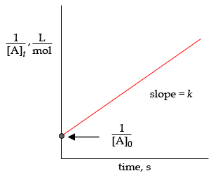
To get the graph of a second-order integrated rate law, rearrange equation #color(blue)((1))# to get
#underbrace(1/([B]))_text(y) = underbrace(k)_text(slope) * t + underbrace(1/([B]_0))_text(y-intercept)#
Your graph will look like this


