What are the mathematical formulations of quantum mechanics?
1 Answer


They are:
- Schrodinger formulation (wave mechanics)
- Heisenberg formulation (matrix mechanics)
- Feynman Path Integral formulation
The major differences are:
- Schrodinger formulated time-dependent wave functions and time-independent operators.
- Heisenberg formulated time-independent ket vectors and time-dependent operators.
- Feynman formulated an integration over all quantum paths, which could be described as the convolution of the Green's function
#G(x,x'; t)# response to an impulse with a weight given by the stationary state#psi(x,t_0)# .
For simplicity we do this in one dimension.
DISCLAIMER: LONG ANSWER!
SCHRODINGER FORMULATION
The time-dependent Schrodinger equation is:
#iℏ(delPsi)/(delt) = hatHPsi# where
#Psi(x,t) = e^(-iEt//ℏ)psi(x)# is the time-dependent wave function and#hatH# is the time-independent Hamiltonian of the system.
As you can see,
- The wave function
#Psi# was time-dependent, but the operators associated with it are time-independent. - The wave function
#psi# was an electric charge density spread out over allspace. - With the input of Max Born,
#psi# is the probability amplitude, while#int_"allspace" psi^"*"psi d tau# is the probability of finding the electron somewhere.
In essence, Schroedinger was a guy who believed in wave mechanics and particle-wave duality, i.e. that quantum particles could be described by the de Broglie relation:
#lambda = h/(mv)#
This is probably the easiest to understand out of all the formulations.
HEISENBERG FORMULATION
Heisenberg, for the life of him, saw it this way:
- A system is described by some arbitrary ket vector
#| n >># , known as a state vector, independent of time. - The inner product of
#| n >># with#<< x |# describing all the possible position bra vectors gives a complete set of eigenstates#<< x | n >> = psi_n(x)# . - The operators could be functions of time, and any time translation operator is unitary.
Under this formulation, the time-dependent Schrodinger equation becomes:
#iℏ (d << x | n >>)/(dt) = hatH << x | n >>#
From this, one could formulate the following relationships:
Overlap of definite position and momentum
#<< x | p_x >> = 1/sqrt(2piℏ) e^(ip_x x//ℏ)#
Matrix product of position and momentum with themselves
#int_(-oo)^(oo)# # | x >> << x |# #dx = int_(-oo)^(oo)# # | p_x >> << p_x |# #dp_x# #-= 1#
Dirac Delta function
#int_(-oo)^(oo) << x | p_x >> << p_x | x' >>dp_x = << x | x' >>#
#= 1/(2piℏ) int_(-oo)^(oo) e^(ip_x(x-x')//ℏ)dp_x = delta(x-x')#
#int_(-oo)^(oo) << p_x | x >> << x | p_x' >>dx = << p_x | p_x' >>#
#= 1/(2piℏ) int_(-oo)^(oo) e^(ix(p_x-p_x')//ℏ)dx = delta(p_x-p_x')#
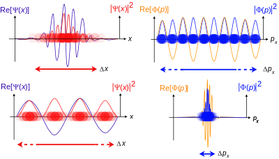
Relation between wave functions in position/momentum representations
#phi_n(p_x) = << p_x | n >>#
#= int_(-oo)^(oo) << p_x | x >> << x | n >> dx#
#= 1/sqrt(2piℏ) int_(-oo)^(oo) e^(-ip_x x//ℏ) psi_n(x) dx#
#psi_n(x) = << x | n >>#
#= int_(-oo)^(oo) << x | p_x >> << p_x | n >> dp_x#
#= 1/sqrt(2piℏ) int_(-oo)^(oo) e^(ip_x x//ℏ) phi_n(p_x) dp_x#
FEYNMAN PATH INTEGRAL FORMULATION
Probably the hardest one to understand, I think... Feynman wanted to describe the transition probability amplitude of the quantum particle by summing over all possible quantum paths:
#| psi (x,t') >># #= int_(-oo)^(oo) << psi(x',t') | psi(x_0, t_0) >> dx' cdot# #| psi(x',t') >>#
Under this formulation, define the unitary time translator
#hatU_t = e^(-ihatH(t-t_0)//ℏ)Theta(t-t_0)# ,where
#Theta(t-t_0) = int_(-oo)^(t) delta(t'-t_0)dt'# is the Heaviside step function and#hatH# is the Hamiltonian of the system.
Then a Green function can be defined in terms of
#G(x,x'; t) = << x | hatU_t | x' >># where
#x'# is the position at which an initial impulse to the system was imparted at time#t_0# , and#x# is the propagated position at time#t# .
The Feynman Path Integral is then the Green's function formulation of a system. For instance, if
#iℏ(delPsi)/(del t) = hatH Psi# ,
then since
#(hatH - iℏ(del)/(delt)) G(x,x'; t)#
#= (hatH - iℏ(del)/(delt)) << x | e^(-ihatH(t-t_0)//ℏ)Theta(t-t_0) | x' >>#
#= [ . . . ] = -iℏ delta(x-x')delta(t-t_0)#
As it turns out, if the Hamiltonian of a system is given by, for example,
#hatH = p_x^2/(2m) + V(hatx)# ,
then for a small enough time step
#G(x,x'; t) = [ . . . ]#
#= 1/(2piℏ) int_(-oo)^(oo) e^(-ip_x^2(t-t_0)//2mNℏ)e^(-iV(hatx)(t-t_0)//Nℏ) e^(ip_x(x-x')//ℏ) dp_x#
#= sqrt((Nm)/(2pi iℏ(t-t_0))) "exp"[(i(t-t_0))/(Nℏ) (N^2/2 m((x - x')/(t-t_0))^2 - V(x'))],#
#N = 1#
This does indeed relate back to the wave function:
#Psi_n(x,t) = int_(-oo)^(oo) underbrace(G(x,x'; t))_(<< x | hatU_t | x' >>) underbrace(psi_n(x',t_0))_(<< x' | n >>) dx'#
In a way (and this made the most sense to me):
The wave function can be given by the integral over the path described by the convolution of the impulse on the system with a weight given by the initial state.
