Question

What is calculus?

Answer 1

Probably not, but here goes! This is First Principles differentiation I will show here. But yeah, this is such a broad question that there is no answer to this question. Don't expect to understand too much of this. Very long answer.

Explanation:

How do you calculate the gradient of a line? How about a curve?

A line is easier, it's simply the change in y over the change of x. A curve is slightly more difficult; the gradient is not constant like with a straight line. Take everyone's favourite curve, `y=x^2`

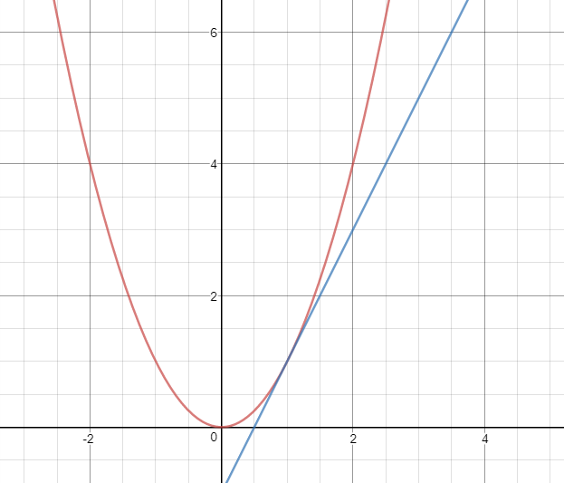
How would we take the gradient at a point, say `(1,1)`? We'd draw a tangent, and take the gradient of the tangent. The problem was, everyone draws slightly different tangents. I might get a gradient of 2.3, you might get 1.9, Jim up the road might get 3.0... there is no way to be certain.

So instead of drawing a tangent, people instead decided to draw chords and took the gradient of the chord.

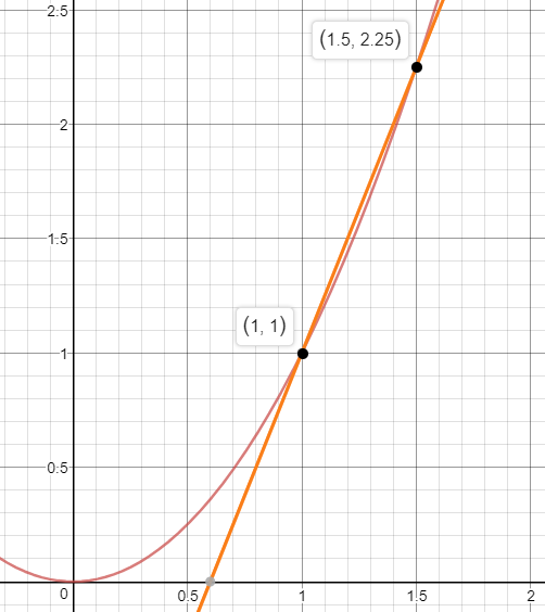
This diagram shows a chord (or technically a secant) passing through the points `(1,1)` and `(3/2,9/4)`. You can calculate that the gradient of this curve is 2.5. But 1.5 is still quite a way away from 1. So let's go closer.

Let `P=(1,1)` and `P'=(1.1, 1.21.)`, both of which are on the curve `y=x^2`
`m_(PP')=(1.21-1)/(1.1-1)`
`=2.1`

We're getting closer and closer to 2, we might begin to suspect that this is 2. We could get closer numerically, x=1.01, 1.001, 1.00000....001 - but this will take forever, and we can do this a better way.
We'll let our co-ordinate by a small change in the x value, denoted by `deltax` (delta x). (Sometimes the letter h is also used)

let `P=(1,1), Q=(1+deltax, (1+deltax)^2)`

grad of `PQ=((1+deltax)^2-1)/(1+deltax-1)`
`=((1+2deltax+deltax^2)-1)/(deltax)`
`=(2deltax+deltax^2)/(deltax)`
`=2+deltax`

But, remember, we were trying to calculate the gradient of a tangent. This only touches the curve at one point, so we would actually be calculating the gradient between `(1,1)` and `(1,1)`
So what we will do is take a limit as `deltax->0` (as delta x approaches 0)

grad of `PQ=lim_(deltax->0)=2+deltax`

`=2`

So the gradient of `y=x^2` at the point (1,1) is 2.

Congratulations!! Now, let's do it for any point of the curve `y=x^2`

Firstly, we will introduce a new notation. This notation is `dy/dx`, which represents the gradient function of `y=`blahblah `x`. Also, `f'(x)` is used to show "the gradient function of `f(x)`.

Let our two points on the curve be `(x,x^2)` and `(x+deltax, (x+deltax)^2)`

`dy/dx=lim_(deltax->0)(((x+deltax)^2-x^2)/(x+deltax-x))`
`=lim_(deltax->0)((x^2+2xdeltax+deltax^2-x^2)/(deltax))`
`=lim_(deltax->0)((2xdeltax+deltax^2)/(deltax))`
`=lim_(deltax->0)(2x+deltax)`
`:. dy/dx=2x` (since this will be true as delta x becomes zero)

Thus, the gradient at any point on the curve `y=x^2` will be `2x`.

In all, the way to find the gradient function of any polynomial `y=f(x)` is:

`dy/dx=lim_(deltax->0)((f(x+deltax)-f(x))/(deltax))`

We can do the same thing for `y=x^3`

`dy/dx=lim_(deltax->0)(((x+deltax)^3-x^3)/(deltax))`
`=lim_(deltax->0)((3x^2deltax+3xdeltax^2+deltax^3)/(deltax))`
`=lim_(deltax->0)(3x^2+3xdeltax+deltax^2)`
`:.dy/dx=3x^2`

You can do the same thing for other polynomials (I won't do them here, but you can in your own time)

`y=x^2 => dy/dx=2x`
`y=x^3 => dy/dx=3x^2`
`y=x^4 => dy/dx=4x^3`
`y=x^5 => dy/dx=5x^4`
`y=x^10 => dy/dx=10x^9`

Notice a pattern?? With binomial theorem as well as first principles, you can show that:

`y=x^n => dy/dx=nx^(n-1)`
`y=kx^n => dy/dx=knx^(n-1)`

Indeed, this isn't all of calculus. Saying this was calculus is like saying all you can do in algebra is sums like `x+2=5`. Nevertheless, I hope this has given you a bit of an insight into this. I'd also recommend this guy and this video; I find he is great for maths stuff general.
)

Answer 2

A calculus and a few thoughts...

Explanation:

This is a calculus...

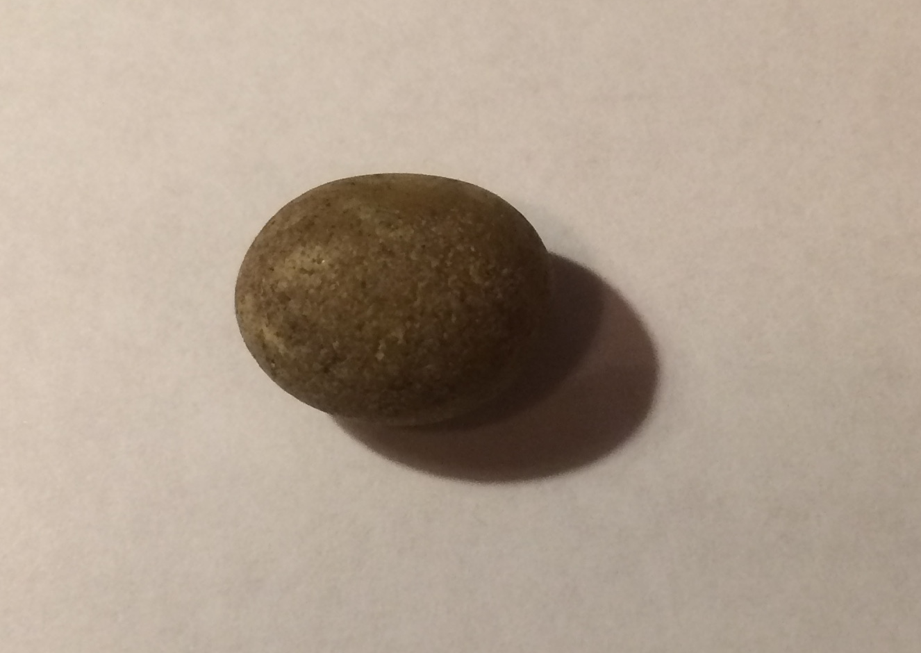
OK, it's a small roundish stone picked up off my driveway, but it could be a calculus. The Latin word calculus refers to a small stone used for counting.

In Calculus, we deal with questions like:

• What is the rate of change of a function at a point?

• What is the area enclosed by a curve?

• What is the average value of a function over a curved surface?

The intuition behind much of calculus goes back to that little stone, or more accurately to infinitesimal quantities.

For example, to find the slope of a function at a point we can look at the slope of secants between points on the graph of that function over an interval that gets smaller and smaller until it is infinitesimally small.

Or to find the area under a curve, we can split the area into smaller and smaller bars (like a histogram) until we have the infinite sum of infinitesimal areas.

To find the average value of a function over a curved surface we can break that surface into smaller and smaller patches, until we have an infinite sum of infinitesimally small patches.

The problem with all this intuitive stuff is that ordinary numbers and arithmetic do not include infinite and infinitesimal quantities. So instead we typically build up a system of methods based on the idea of limits.

For example, the rate of change, instantaneous slope or derivative of a function `f(x)` at a point `a` is given by:

`f'(a) = lim_(h->0) (f(a+h)-f(a))/h`

If you look closely, you will see that this is:

`lim_(h->0) (f(a+h)-f(a))/((a+h)-a)`

which is the limit of the slope of the secant of the function `f(x)` in the interval `[a, a+h]`. That is, it is the limit of the slope of the line between `(a, f(a))` and `(a+h, f(a+h))` as `h->0`.

I have only touched the tiniest fragment of what Calculus is about here, but start from the intuition and it may make more sense than going straight for formulas.