Question

Consider Hydrogen ion in a box having one dimension, then find electron probability distribution?

Answer 1

`psi_n^"*"(x)psi_n(x) = 2/L sin^2((npix)/L)`

These solutions are well-known and you should get to know what they look like. Here are the wave function `psi` and the probability density `psi_n^"*"psi_n` plotted:

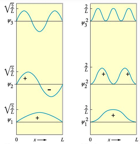
Also, on the side, we got that `k = npi"/"L`, so since

`k = (npi)/L = sqrt((2mE)/ℏ^2)`,

it follows that the energy levels are given by:

`color(blue)(E_n) = (ℏ^2k^2)/(2mL^2) = color(blue)((ℏ^2n^2pi^2)/(2mL^2))`

---

DISCLAIMER: LONG ANSWER!

A hydrogen cation (presumably `""^(1) "H"^(+)`) is a neutron and proton with no potential of interaction. Thus, we set this up as a particle in a box scenario where `V = 0`.

The Hamiltonian for such a scenario is:

`hatH = hatK + cancel(hatV)^(0)`

`= -ℏ^2/(2m) (del^2)/(delx^2)`

The box looks like:

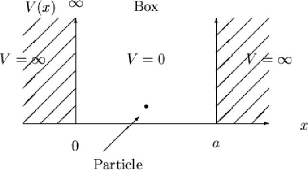
with boundary conditions `psi(0) = psi(L) = 0`, and

`V = {(0, x in (0,L)),(oo, x <= 0),(,x >= L):}`

The Schrodinger equation is then:

`hatHpsi = Epsi`

`=> -ℏ^2/(2m) (d^2psi)/(dx^2) = Epsi`

Rearrange to the standard form:

`(d^2psi)/(dx^2) + (2mE)/(ℏ^2)psi = 0`

Often we set the substitution `k = sqrt(2mE//ℏ^2)`, so

`(d^2psi)/(dx^2) + k^2psi = 0`

The general solution to this is assumed to be

`psi = e^(rx)`

and upon inserting it, we obtain the auxiliary equation:

`r^2 e^(rx) + k^2 e^(rx) = 0`

In the well, `e^(rx) ne 0` so that the particle exists. Thus,

`r = ik`

and we write a linear combination for `psi`:

`psi = c_1e^(ikx) + c_2e^(-ikx)`

Using Euler's formula, we rewrite this in terms of real trig functions.

`psi = c_1(cos(kx) + isin(kx)) + c_2(cos(kx) - isin(kx))`

`= (c_1 + c_2)cos(kx) + (ic_1 - ic_2)sin(kx)`

Define `A = c_1 + c_2` and `B = ic_1 - ic_2`, because these are arbitrary constants. Therefore:

`psi = Acos(kx) + Bsin(kx)`

The boundary conditions state that since the potential goes to `oo` at `x = 0,L`, it follows that `psi(0) = psi(L) = 0`:

`Acos(kcdot0) + Bsin(kcdot0) = Acos(kL) + Bsin(kL) = 0`

But since `sin(0) = 0` and `cos(0) = 1`, it follows that `A = 0`. Furthermore, since `A = 0`, we have:

`Bsin(kL) = 0`

And this is only when `kL = npi`, where `n = 1, 2, 3, . . .`. (We could take negative `n`, but that would give a linearly dependent solution.)

Thus, since `k = (npi)/L`, the wave function becomes:

`psi_n(x) = Bsin((npix)/L)`

And the probability distribution is then:

`psi_n^"*"(x)psi_n(x) = B^2 sin^2((npix)/L)`

A well-behaved wave function is normalized in its boundaries, so we say that

`int_(0)^(L) psi_n^"*"psi_ndx = 1`

From this we get the normalization constant.

`1 = B^2 int_(0)^(L) sin^2((npix)/L)dx`

Consider the following argument.

If `sin^2u + cos^2u = 1`, then integrating `sin^2u + cos^2u` gives `L` for the area under the curve, with height `1` and length `L`, regardless of what `u` is.

The identities `sin^2u = 1/2(1-cos(2u))` and `cos^2u = 1/2(1+cos(2u))` show that `sin^2u` contributes to half the area under the curve.

Therefore, `int_(0)^(L) sin^2udu = L/2`, and `B = sqrt(2/L)`. This means

`color(blue)(psi_n^"*"(x)psi_n(x) = "Probability Distribution")`

`= color(blue)(2/L sin^2((npix)/L))`