Question

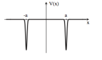
How do I plot the energy eigenvalues and wave function solutions of a delta function double potential well with `V(chi) = -alpha(delta(chi+L)+delta(chi-L))`?

Answer 1

Well, here it is... Here is the Excel sheet I made while doing this. Also, here are the even solution graphs.

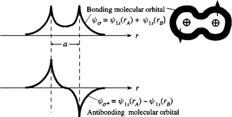
This, by the way, results in a wave function solution that resembles the hydrogen molecule, except with internuclear distance `a = 2L`, and our solution is horizontally flipped:

This is the case because `psi` for a `1s` orbital behaves similarly to a `delta` function at a nucleus, except the function is wider.

---

DISCLAIMER: VERY LONG ANSWER!

Here's the scenario (just change `a->L`):

We set up the wave function for a tunnelling free-particle. Call the regions `I`, `II`, and `III` from left to right. Before we use any boundary conditions:

`psi_I = Ae^(-kchi) + Be^(kchi)`
`psi_(II) = Ce^(-kchi) + De^(kchi)`
`psi_(III) = Fe^(-kchi) + Ge^(kchi)`

where `k = sqrt(-(2mE)/ℏ^2)`, since `E < 0` for bound states.

Since the wave function must vanish at `chi -> pm oo`, `A = 0` and `G = 0`. Due to the even symmetry of the Dirac Delta function,

• `C = D` for even solutions and `C = -D` for odd solutions.
• `G = B` for even solutions and `G = -B` for odd solutions.

This simplifies down to even solutions being:

`psi_"even" = {(Be^(kchi),-oo < chi < -L),(C(e^(-kchi) + e^(kchi)),-L < chi < L),(Be^(-kchi),L < chi < oo):}`

and odd solutions being:

`psi_"odd" = {(-Be^(kchi),-oo < chi < -L),(C(e^(-kchi) - e^(kchi)),-L < chi < L),(Be^(-kchi),L < chi < oo):}`

EVEN SOLUTION

Continuity at `chi = -L` gives:

`Be^(-kL) = C(e^(kL) + e^(-kL))`

`=> B = C(e^(2kL) + 1)`

Next, consider the Schrodinger equation at just `chi = -L`:

`-ℏ^2/(2m) (d^2psi)/(dchi^2) - alphadelta(chi+L)psi = Epsi`

Integration near `chi = -L` only gives:

`-ℏ^2/(2m) lim_(epsilon->0) int_(-L-epsilon)^(-L + epsilon) (d^2psi)/(dchi^2) dchi - alpha lim_(epsilon->0) int_(-L-epsilon)^(-L+epsilon) delta(chi+L)psidchi = lim_(epsilon -> 0) Eint_(-L-epsilon)^(-L+epsilon) psidchi`

Denote `Lpm epsilon = L^(pm)` to make this easier to read. Integrating a constant of infinitely small width gives zero:

`-ℏ^2/(2m) int_(-L^(-))^(-L^(+)) (d^2psi)/(dchi^2) dchi - alpha int_(-L^(-))^(-L^(+)) delta(chi+L)psidchi = 0`

Evaluating the integrals requires examination of the left and right sides of the discontinuous derivative.

`-ℏ^2/(2m) (Delta (dpsi(-L))/(dchi)) = alpha psi(-L^(pm))`

Now evaluate the `psi` and its derivatives at `-L` either from the left or right of the `delta` potential.

`-ℏ^2/(2m) (-kCe^(kL) + kCe^(-kL) - kBe^(-kL)) = alpha Be^(-kL)`

`C(-e^(kL) + e^(-kL)) - Be^(-kL) = -(2malpha)/(ℏ^2k) Be^(-kL)`

Multiply through by `e^(kL)` and rearrange to get:

`C(-e^(2kL) + 1) = B - (2malpha)/(ℏ^2k) B`

`C(e^(2kL) - 1) = B((2malpha)/(ℏ^2k) - 1)`

Seeing as we have an expression for `B` already, solve for `e^(-2kL)` on one side.

`cancelC(e^(2kL) - 1) = cancelC(e^(2kL) + 1)((2malpha)/(ℏ^2k) - 1)`

`e^(2kL) - 1 = (2malpha)/(ℏ^2k)e^(2kL) - e^(2kL) + (2malpha)/(ℏ^2k) - 1`

`e^(2kL) = ((2malpha)/(ℏ^2k) - 1)e^(2kL) + (2malpha)/(ℏ^2k)`

`1 = (2malpha)/(ℏ^2k) - 1 + (2malpha)/(ℏ^2k)e^(-2kL)`

`cancel2(1 - (malpha)/(ℏ^2k)) = cancel2[(malpha)/(ℏ^2k)e^(-2kL)]`

`color(blue)(e^(-2kL) = (ℏ^2k)/(malpha) - 1)`

Let `x = 2kL` and `c = (ℏ^2)/(2mLalpha)`. Note: `x ne chi`. This results in plotting `e^(-x)` vs. `cx - 1`. If `alpha = ℏ^2/(2mL)`, then `c = 1`. So let's take `c = 1, 0.75`:

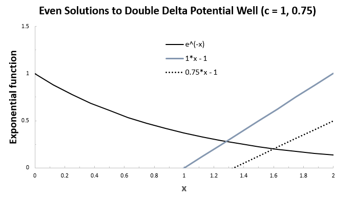
Clearly, there will always be an intersection (always at least one bound state) as long as `c` is nonsmall, because we are looking at a decreasing function intersecting with an increasing function of slope `c` at positive `x`.

The x-intercept turns out to be `1//c`, and the intersection occurs at `x ~~ 1.27846` for `c = 1`.

So the approximate even solution energy for `c = 1` is:

`1.27846 ~~ 2kL`

`=> k^2 ~~ 0.40861/L^2 = -(2mE)/(ℏ^2)`

`=> color(blue)(E ~~ -(0.20431ℏ^2)/(mL^2))`

If we take the limit as `c -> 0`, i.e. the limit as `alpha -> oo`, no bound state exists (no intersection found), so we want `0 < alpha < ℏ^2/(2mL)`.

ODD SOLUTION

Continuity at `chi = L` again gives:

`Be^(-kL) = C(e^(-kL) - e^(kL))`

`=> B = -C(e^(2kL) - 1)`

As before, consider the Schrodinger equation at just `chi = L`:

`-ℏ^2/(2m) (d^2psi)/(dchi^2) - alphadelta(chi-L)psi = Epsi`

Integration near `chi = +L` only gives:

`-ℏ^2/(2m) int_(L^(-))^(L^(+)) (d^2psi)/(dchi^2) dchi - alpha int_(L^(-))^(L^(+)) delta(chi-L)psi = 0`

As before, we now get:

`-ℏ^2/(2m) (Delta (dpsi(L))/(dchi)) = alpha psi(L^(pm))`

Now evaluate the `psi` and its derivatives at `L` either from the left or right of the `delta` potential.

`-ℏ^2/(2m) (-kBe^(-kL) + kCe^(-kL) + kCe^(kL)) = alpha Be^(-kL)`

`(ℏ^2k)/(2malpha) (Be^(-kL) - Ce^(-kL) - Ce^(kL)) = Be^(-kL)`

Again multiply through by `e^(kL)` to solve:

`(ℏ^2k)/(2malpha) (B - C - Ce^(2kL)) = B`

`(ℏ^2k)/(2malpha) (-C - Ce^(2kL)) = B(1 - (ℏ^2k)/(2malpha))`

`(ℏ^2k)/(2malpha) C(1 + e^(2kL)) = B((ℏ^2k)/(2malpha) - 1)`

`C(1 + e^(2kL)) = B(1 - (2malpha)/(ℏ^2k))`

Now plug in `B = -C(e^(2kL) - 1)`:

`cancelC(1 + e^(2kL)) = cancelC(1 - e^(2kL))(1 - (2malpha)/(ℏ^2k))`

`1 + e^(2kL) = 1 - (2malpha)/(ℏ^2k) - e^(2kL) + e^(2kL)(2malpha)/(ℏ^2k)`

`cancel2e^(2kL) - e^(2kL)(cancel2malpha)/(ℏ^2k) = - (cancel2malpha)/(ℏ^2k)`

`1 - (malpha)/(ℏ^2k) = - (malpha)/(ℏ^2k)e^(-2kL)`

`color(blue)(e^(-2kL) = 1 - (ℏ^2k)/(malpha))`

Now we again let `x = 2kL` (again, note: `x ne chi`) and `c = (ℏ^2)/(2mLalpha)`. This results in plotting `e^(-x)` vs. `1 - cx`. If `alpha = ℏ^2/(2mL)`, then `c = 1`, so let `c = 1, 0.5`. This gives:

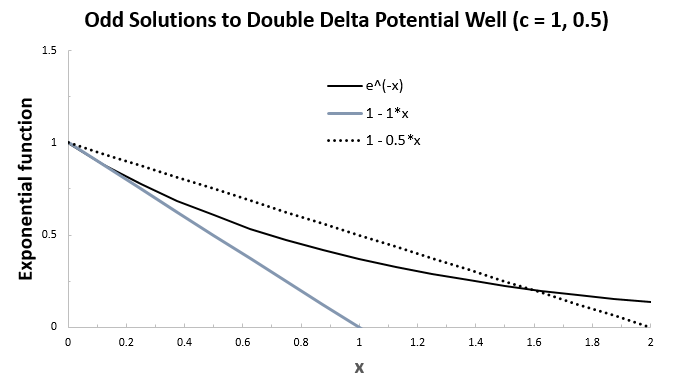
The y-intercept turns out to be `1//c`, and the intersection occurs only for `c < 1` or `alpha > ℏ^2/(2mL)`.

HOW DO THE WAVE FUNCTIONS LOOK?

We'll get two bound states if `c < 1`, and only one if `c >= 1`. For the rest of this answer, I choose `bb(L = 2)`.

The even solution energy for `c = 0.5` (intersection at `x ~~ 2.21772`) is:

`2.21772 ~~ 2kL`

`=> k^2 ~~ 1.22957/L^2 = -(2mE)/(ℏ^2)`

`=> color(blue)(E ~~ -(0.61479ℏ^2)/(mL^2))`

In this case we can then get `k` and then plug it back into the wave function. Here is the even solution:

`k = sqrt(-(2m)/ℏ^2 cdot -(0.61479ℏ^2)/(mL^2))`

`= sqrt(2 cdot (0.61479)/(L^2)) = 1.10886/L`

where I simply chose `B = 1` and `C = 0.0981705` to match `psi` at the boundaries.

`=> psi_(I) = Be^(1.10886x//L)`
`=> psi_(II) = C(e^(-1.10886x//L) + e^(1.10886x//L))`
`=> psi_(III) = Be^(-1.10886x//L)`

This results in (the `x` axis plots `chi`):

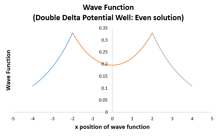
This looks remarkably like the hydrogen bonding molecular orbital wave function plot!

Then, we get `x ~~ 1.59362` for the intersection in the corresponding odd solution. So the approximate odd solution energy for `c = 0.5` is:

`1.59362 ~~ 2kL`

`=> k^2 ~~ 0.63491/L^2 = -(2mE)/(ℏ^2)`

`=> color(blue)(E ~~ -(0.31745ℏ^2)/(mL^2))`

The other bound state (odd solution) has:

`k = sqrt(-(2m)/ℏ^2 cdot -(0.31745ℏ^2)/(mL^2))`

`= sqrt(2 cdot (0.31745)/(L^2)) = 0.79681/L`

`=> psi_(I) = -Be^(0.79681x//L)`
`=> psi_(II) = C(e^(-0.79681x//L) - e^(0.79681x//L))`
`=> psi_(III) = Be^(-0.79681x//L)`

Here I just chose `B = 1` and matched `psi` at the boundaries to get `C = -0.254998` as before. The scale of this need not match the other solution.

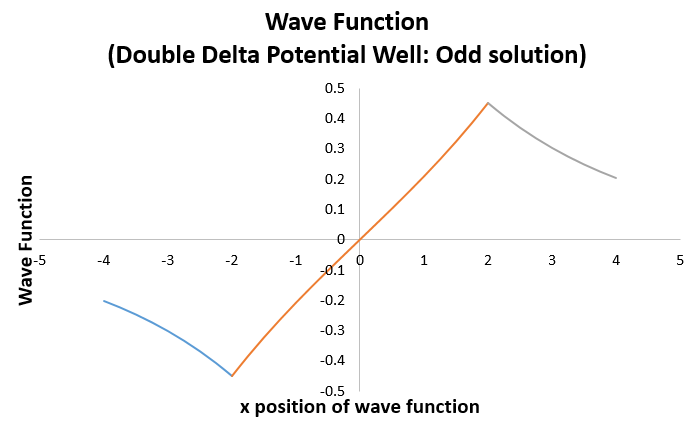
which looks like the hydrogen antibonding molecular orbital wave function plot!

(Again, the `x` axis plots `chi`, the wave function position.)

---

What if we choose `c = 2`? The even solution and odd solution have intersections at `x ~~ 0.73884` and `x ~~ -1.25643`, respectively. Here's the problem...

If `x < 0`, then `2kL < 0`. We must have `L > 0`, so that would imply that `k < 0`, whereas we defined `k = sqrt(-(2mE)/ℏ^2) > 0`.

Hence, we discard the odd solution and only have an even solution:

`0.73884 ~~ 2kL`

`=> k^2 ~~ 0.13647/L^2 = -(2mE)/(ℏ^2)`

`=> color(blue)(E ~~ -(0.06824ℏ^2)/(mL^2))`

With this scenario,

`k = sqrt(-(2m)/ℏ^2 cdot -(0.06824ℏ^2)/(mL^2))`

`= sqrt(2 cdot (0.06824)/(L^2)) = 0.36943/L`

You can plug it back in if you wish, but I'm not going to plot this one, because it's unphysical; since this entire problem can be used to model something not unlike `"H"_2` molecular orbitals, having a bonding MO (even solution) but no antibonding MO (odd solution) doesn't make physical sense.