What is the change in the object’s velocity from t=4 to t=10?
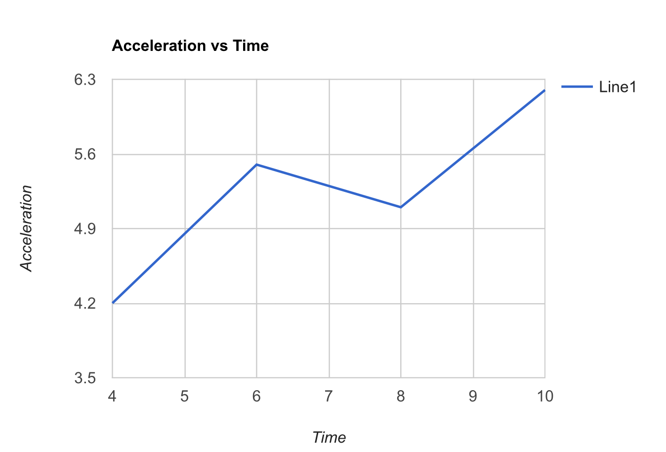
The acceleration of an object at various times is shown in the table below. Using the information in the table, estimate the change in the object’s velocity from t=4 to t=10.

The acceleration of an object at various times is shown in the table below. Using the information in the table, estimate the change in the object’s velocity from t=4 to t=10.
2 Answers
- Assuming that acceleration changes from
t=4t=4 tot=6t=6 linearly, we see thatdot a=(5.5-4.2)/2=0.65\ ms^-3
Integrating both sides with respect to time we get
a=0.65t+C ......(1)
whereC is a constant of integration to be evaluated from initial conditions. It is given that att=4=>t_0=0, a=4.2 . Inserting in (1) we get
4.2=0.65xx0+C
=>C=4.2
Inserting in (1) we get
a=0.65t+4.2 .......(2)
We know thata=dot v . Integrating with respect to time both sides we get
v=int(0.65t+1.6)\ dt
=>v=0.65t^2/2+4.2t+C_1 .....(3)
whereC_1 is a constant of integration to be evaluated from initial conditions. Let us assume that att=4=>t_0=0, v=v_4 . Inserting in (3) we get
=>v_4=0.65xx0^2/2+4.2xx0+C_1
=>C_1=v_4
Inserting in (3) we get
=>v=0.325t^2+4.2t+v_4
calculating velocity att=6=> this acceleration was in operation for2s
v_6=0.325xx2^2+4.2xx2+v_4
=>v_6=9.7+v_4 .........(4) - Assuming that acceleration changes from
t=6 tot=8 linearly, we see that for this time intervaldot a=(5.1-5.5)/2=-0.2\ ms^-3
Integrating both sides with respect to time we get
a=-0.2t+C_2 ......(5)
whereC_2 is a constant of integration to be evaluated from initial conditions. It is given that att=6=>t_0=0, a=5.5 . Inserting in (5) we get
5.5=-0.2xx0+C_2
=>C_2=5.5
Inserting in (5) we get
a=-0.2t+5.5 .......(6)
We know thata=dot v . Integrating with respect to time both sides we get
v=int(-0.2t+5.5)\ dt
=>v=-0.1t^2+5.5t+C_3 .....(7)
whereC_3 is a constant of integration to be evaluated from initial conditions. We have att=6=>t_0=0, v_6=9.6+v_4 . Inserting in (3) we get
=>9.6+v_4=-0.1xx0^2+5.5xx0+C_3
=>C_3=9.6+v_4
Inserting in (7) we get
=>v=-0.1t^2+5.5t+9.6+v_4
calculating velocity att=8=> this acceleration was in effect for2s
v_8=-0.1xx2^2+5.5xx2+9.6+v_4
=>v_8=20.2+v_4 .........(8) - Assuming that acceleration changes from
t=8 tot=10 linearly, we see thatdot a=(6.2-5.1)/2=0.55\ ms^-3
Integrating both sides with respect to time we get
a=0.55t+C_4 ......(9)
whereC_4 is a constant of integration to be evaluated from initial conditions. It is given that att=8=>t_0=0, a=5.1 . Inserting in (9) we get
5.1=0.55xx0+C_4
=>C_4=5.1
Inserting in (9) we get
a=0.55t+5.1 .......(10)
We know thata=dot v . Integrating with respect to time both sides we get
v=int(0.55t+5.1)\ dt
=>v=0.55t^2/2+5.1t+C_5 .....(11)
whereC_5 is a constant of integration to be evaluated from initial conditions. We have calculated that att=8=>t_0=0, v_8=20.2+v_4 . Inserting in (11) we get
=>20.2+v_4=0.55xx0^2/2+5.1xx0+C_5
=>C_5=20.2+v_4
Inserting in (11) we get
=>v=0.275t^2+5.1t+20.2+v_4
calculating velocity att=10=> this acceleration was in operation for2s
v_10=0.275xx2^2+5.1xx2+20.4+v_4
=>v_10=(31.7+v_4)\ ms^-1 .........(12)

Explanation:
Acceleration is given by
"a" = "Δv"/"t"
"Δv = at"
From above equation we can say that area of an acceleration vs time graph gives us change in velocity.
Acceleration vs Time graph from
Area under this graph is change in velocity of object
-
From
t = 4 tot =6
"Δv"_1 = [1/2 × 2 × (5.5 - 4.2)] + [(6 - 4) × (4.2 - 3.5)]
color(white)(Δv_1) = 1.3 + 1.4
color(white)(Δv_1) = "2.7 m/s" -
From
t = 6 tot = 8
"Δv"_2 = [1/2 × 2 × (5.5 - 5.1)] + [(8 - 6) × (5.1 - 3.5)]
color(white)(Δv_2) = 0.4 + 3.2
color(white)(Δv_2) = "3.6 m/s" -
From
t = 8 tot = 10
"Δv"_3 = [1/2 × 2 × (6.2 - 5.1)] + [(10 - 8) × (5.1 - 3.5)]
color(white)(Δv_3) = 1.1 + 3.2
color(white)(Δv_3) = 4.3\ "m/s"
Change in velocity from
