A quantity decades exponentially if it decreases in time at a rate that is linearly proportional to its value. In terms of equations, if #y# decays exponentially, then #dy/dt = - k y#, where #k>0# is the exponential decay constant and it characterizes the decay.
The variables involved in this differential equation are separable. If we separate them, we get #1/y dy = -k dt#. Now we can integrate:
#ln(y)=-kt+tilde{c}#
where #tilde{c}# is a constant. In the end: #y(t)=ce^{-kt}#, where #c=e^{tilde{c]}>0#.
This means that graphing the exponential decay turns into graphing an exponential function with negative exponent. For #t=0# (the instant in which the decay starts), we get that #y_0=y(0)=c#. So the parameter #c# is the #y#-intercept of the function: it represents the value of our quantity #y# at the instant in which the decay starts.
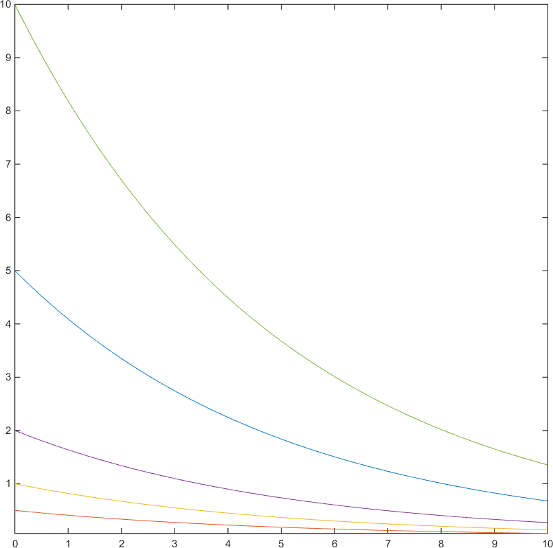
We can plot #y(t)# for some values of #c#. In the following plot #k=0.2# and different colors represent graphs for #c=10#, #c=5#, #c=2#, #c=1# and #c=0.5# (from the top to the bottom).
To get a visual intuition of what the differential equation #dy/dt=-ky# really means, let's consider the #(t,y)#-plane. We are indeed interested in the behavior of the quantity #y# in time #t#.
If we fix a point #(t_p,y_p)# on the plane, we are stating that the quantity #y# has the value #y=y_p# at time #t=t_p#. We want to represent the decay, so we ask ourselves where would the point #(t_p,y_p)# "decay" after a "bit" of time. This "bit" can be thought as infinitesimally small: we denote it by #(dt)_p#. In this infinitesimal time, the quantity #y# changes by an infinitesimally small amount #(dy)_p#.
So, the point we are searching for is the point #(t_p+(dt)_p,y_p+(dy)_p)#, which is the point that is going to describe the decay an infinitesimal amount of time after #t_p#. To represent this information we draw an arrow (namely a vector) in #(t_p,y_p)#, pointing in the direction of #(t_p+(dt)_p,y_p+(dy)_p)#. The vector's direction is given by the difference
#(t_p+(dt)_p,y_p+(dy)_p)-(t_p,y_p)=((dt)_p,(dy)_p)#
From the differential equation we get that #((dt)_p,(dy)_p)=((dt)_p,-ky_p(dt)_p)#. Now we can choose the size of the arrow by setting #(dt)_p# as small as we like.
[This argument is not rigorous: we should speak about finite differences and how they are related to differentials, but the core idea emerges anyway. Also notation is invented for the purpose of the argument.]
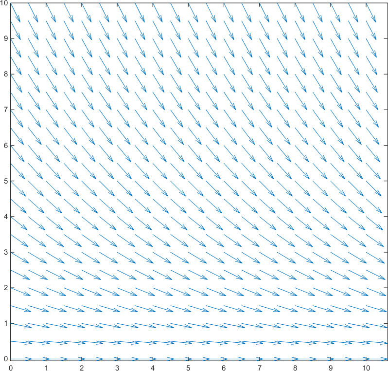
If we repeat this operation for some points, we get the following picture. Note that vectors are normalized (i.e. made unitary dividing by their norm) and this particular plot is made fixing #k=0.2# (other positive values of #k# don't change the qualitative behavior).
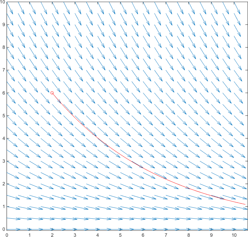
Now, given any point #(t_p,y_p)#, we are "forced" to follow the arrows and we get the plot of the decay when the quantity #y# has value #y_p# at time #t=t_p#. In the following picture I chose #(t_p,y_p)=(2,6)# and #k=0.2# as in the previous examples.