Let's recall composite Simpson's rule: if nn is a even positive integer and f(x)f(x) is an integrable function over the closed finite real interval [a,b][a,b], then
int_a^b f(x) dx approx h/3 sum_{j=1}^{n/2}[f(x_{2j-2})+4f(x_{2j-1})+f(x_{2j})]∫baf(x)dx≈h3n2∑j=1[f(x2j−2)+4f(x2j−1)+f(x2j)]
where h=(b-a)/nh=b−an and x_j=a+jhxj=a+jh for j=0,ldots,n.
What this rule really does is splitting the interval I=[a,b] in n/2 subintervals I_k=[x_{2k-2},x_{2k}], for k=1,ldots,n/2. The diameter of I_k for all k=1,ldots,n/2 is equal to 2h, and the formula approximates the integral on each I_k using (simple) Simpson's rule. Then, we sum up the results (additive property of the integral) and get the composite approximation.
High values of n lead to better the approximation, as the error is bounded by the following function of h (that is inversely proportional to n):
|epsilon| le h^4/180 (b-a) max_{c in [a,b]} |f^((4)) (c)|
Note 1: this requires that our function is differentiable 4 times on [a,b], and this regularity is not guaranteed.
Note 2: when integrating numerically, estimating error is not an option. If we are not able to bound error, it might be very high and the result may be very highly imprecise.
In our case [a,b]= [0,2], f(x)=sqrt(x) * e^{-x} (which is continuous on [0,2] and therefor integrable on [0,2]) and n=10, so h=(2-0)/10=1/5. We get x_0=0, x_1=0.2, x_2=0.4, x_3=0.6, x_4=0.8, x_5=1 , x_6=1.2, x_7=1.4, x_8=1.6, x_9=1.8 and x_10=2.
if we denote y_j=f(x_j) for all j=0,...,10, then y_0=0, y_1 approx 0.3661, y_2 approx 0.4239, y_3 approx 0.4251, y_4 approx 0.4019, y_5 approx 0.3679, y_6 approx 0.3299, y_7 approx 0.2918, y_8 approx 0.2554, y_9 approx 0.2218 and y_{10}=0.1914.
To get our approximation of the integral, we have to compute the following summation:
h/3 sum_{k=1}^{n/2}[y_{2k-2}+4y_{2k-1}+y_{2k}] =1/15[y_0 + 4y_1+2y_2+4y_3+2y_4+4y_5+2y_6+4y_7+2y_8+4y_9+y_10] approx 9.7044/15 approx 0.6470
In the end we get that int_0^2 sqrt(x) * e^{-x} dx approx 0.6470.
Now we have to find out some bounds for error epsilon, to guarantee some degree of precision. We try with the formula given above. First of all, we have to compute f^((4))
f^((1)) (x)=(e^(-x) (1-2 x))/(2 sqrt(x))
f^((2))(x)= (e^(-x) (4 x^2-4 x-1))/(4 x^(3/2))
f^((3))(x)=(e^(-x) (3+6 x+12 x^2-8 x^3))/(8 x^(5/2))
f^((4))(x)=(e^(-x) (-15-24 x-24 x^2-32 x^3+16 x^4))/(16 x^(7/2))
Here's the graph of |f^((4))|:
graph{|(e^(-x) (-15-24 x-24 x^2-32 x^3+16 x^4))/(16 x^(7/2))| [-0.1, 2.1, -5, 50]}
as we can easily guess from this graph, in [0,2] there's no (finite) maximum value for this function. In fact
lim_{x to 0} |f^((4))(x)|=lim_{x to 0} 15/(16 x^(7/2))=+infty
Using the estimate given above (considering supremum instead of maximum), we get that |epsilon| le +infty, which is not a great discovery. So we can't conclude anything about the precision of our result using this estimate (in general no estimates involving derivatives could ever work, as all derivatives of this function diverge for x to 0).
However we should not give up. The following is a plot of the function f(x) (black curve) and of the interpolating parabolas P_k(x) (red curves) used to approximate f(x) on the I_k intervals in Simpson's formula. The green curves represent the absolute values of errors |E_k(x)|=|P_k(x)-f(x)| made in approximating f(x) on I_k with the P_k(x)s, for k=1,ldots,n/2.
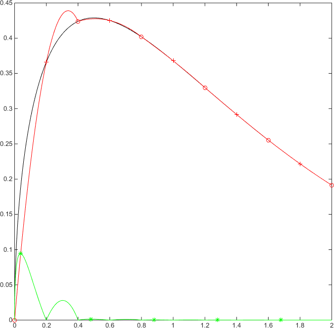
This graph suggests that the integrals of the |E_k(x)|s are finite, even in a neighborhood of 0. For k=1,ldots,n/2
|epsilon_k|=|int_{x_{2k-2}}^{x_{2k}}[P_k(x)-f(x)]dx| le int_{x_{2k-2}}^{x_{2k}}|P_k(x)-f(x)|dx=int_{x_{2k-2}}^{x_{2k}}|E_k(x)|dx le 2h max_{xi in [x_{2k-2},x_{2k}]} |E_k(xi)|
where the last inequality is obtained considering that the area of the rectangle bounding |E_k(x)|'s graph on I_k exceeds the value of the integral (which represents the area bounded by the graph and the x axis).
As already recalled above, composite Simpson's rule is the sum of (simple) Simpson's rule applied on the I_ks. So error epsilon is the sum of errors epsilon_k
|epsilon| =|sum_{k=1}^{n/2} epsilon_k| le sum_{k=1}^{n/2} |epsilon_k|, where k=1,ldots,n/2
In our case, problems arise only in a (right) neighborhood of 0, so in estimating epsilon_1. Let's try to work on it separately and to apply the "classic" error estimate for the other ones:
|epsilon_k| le h^5/80 max_{c_k in [x_{2k-2},x_{2k}]} |f^((4))(c_k)| for k=2,3,4,5.
Considering that |f^((4))(x)| is a constantly decreasing function (so its maximum on a closed interval is the left extreme), we get the following values
|epsilon_2| le (0.2)^5/80 |f^((4))(0.4)| < 4*10^{-6} * 31.133 =124.532 * 10^{-6}
|epsilon_3| le (0.2)^5/80 |f^((4))(0.8)| < 4*10^{-6} * 3.643 =14.572 * 10^{-6}
|epsilon_4| le (0.2)^5/80 |f^((4))(1.2)| < 4*10^{-6} * 1.000 =4.000 * 10^{-6}
|epsilon_5| le (0.2)^5/80 |f^((4))(1.6)| < 4*10^{-6} * 0.344 = 1.376 * 10^{-6}
For |epsilon_1| we consider the bounding rectangle of the graph of |E_1(x)| on I_1: epsilon_1 le 0.4 max_{xi in [0,0.4]} |E_1(xi)|.
So we have to compute the expression of P_1(x) and maximize |E_1(x)|.
P_1(x)=y_0/(2h^2) (x-x_1)(x-x_2)-y_1/h^2 (x-x_0)(x-x_2)+y_2/(2h^2)(x-x_0)(x-x_1)=5 sqrt(5)e^(-2/5) (sqrt(2)/2-e^(1/5))x^2 +sqrt(5)e^(-2/5) (2e^(1/5)-sqrt(2)/2) x
so
|E_1(x)|=|5 sqrt(5)e^(-2/5) (sqrt(2)/2-e^(1/5))x^2 +sqrt(5)e^(-2/5) (2e^(1/5)-sqrt(2)/2) x-sqrt(x)*e^(-x)|
To maximize this, we proceed graphically: we plot |E_1(x)| and find an upper bound for |E_1(x)| as x in [0,0.4]. Other techniques require too much calculations and this answer is long enough. Of course, the result is not rigorous and should be proved.
graph{|5 sqrt(5)e^(-2/5) (sqrt(2)/2-e^(1/5))x^2 +sqrt(5)e^(-2/5) (2e^(1/5)-sqrt(2)/2) x-sqrt(x)*e^(-x)| [-0.05, 0.45, -0.01, 0.15]}
We observe that |E_1(x)| < 0.1 for x in [0,0.4], so |epsilon_1|<0.4*0.1=4 * 10^{-2}.
So in the end we have
|epsilon| le |epsilon_1|+|epsilon_2+|epsilon_3|+|epsilon_4|+|epsilon_5| < 4*10^{-2}+124.532 * 10^{-6}+14.572 * 10^{-6}+4 * 10^{-6}+1.376 * 10^{-6}<0.180484
This result is not satisfactory: the real error is much smaller than this.