How do you minimize and maximize #f(x,y)=x^2+y^3# constrained to #0<x+3y<2#?

2 Answers
Dec 22, 2016

Constrain even more to #x+3y = 1#. Then we can treat this as a cubic in #y#, therefore unbounded.

Explanation:

Suppose we constrain #x+3y = 1#. Then #f(x, y)# is still unbounded:

#f(x, y) = x^2+y^3 = (1-3y)^2+y^3 = y^3+9y^2-6y+1#

The end behaviour is dominated by the #y^3# term and hence:

#lim_(y->+oo) f(x, y) = +oo#

#lim_(y->-oo) f(x, y) = -oo#

Dec 22, 2016

See below.

Explanation:

Given #f(x,y)=x^2+y^3# subjected to #Omega(x,y)#

#Omega(x,y) ={ (x,y) | 0 < x+3y < 2}#

We are looking for local minima/maxima.

This problem can be handled using lagrange multipliers. This can be done following the steps:

1) Describe #Omega(x,y)# through equality constraints
This can be done introducing the so called slack variables #s_1,s_2# and making

#g_1(x,y,s_1) = x + 3y - s_1^2=0#
#g_2(x,y,s_2) = x + 3y - 2+ s_2^2=0#

then #Omega(x,y) equiv g_1(x,y,s_1) nn g_2(x,y,s_2)#

2) Form the Lagrangian

#L(x,y,s_1,s_2,lambda_1,lambda_2)=f(x,y)+lambda_1g_1(x,y,s_1)+lambda_2 g_2(x,y,s_2)#

3) Determine the stationary points of #L(x,y,s_1,s_2,lambda_1,lambda_2)#

This is done computing the solution to

#grad L(x,y,s_1,s_2,lambda_1,lambda_2) = vec 0#

where #grad# represents the partial derivatives operator

#grad = (partial/(partial x),partial/(partial y),partial/(partial s_1),partial/(partial s_2),partial/(partial lambda_1),partial/(partial lambda_2))#

so the equations which define the stationary points are

#{ (lambda_1 + lambda_2 + 2 x = 0), (3 lambda_1 + 3 lambda_2 + 3 y^2 = 0), (2 lambda_1 s_1 =0), (2 lambda_2 s_2 = 0), ( x + 3 y-s_1^2 = 0), (x + 3 y-2 + s_2^2 = 0):}#

Solving for #x,y,s_1,s_2,lambda_1,lambda_2# we obtain

#((x,y,s_1,s_2,lambda_1,lambda_2),(18., -6., 0, -1.41, -36., 0), (0, 0, 0, -1.41, 0, 0), (21.81, -6.60,-1.41, 0, 0, -43.63), (0.183, 0.60, -1.41, 0, 0, -0.36))#

4) Qualifying the stationary points

This can be done computing #(d^2(f @ g_i))/(dx^2)# for #i=1,2#

and depending on the sign, if positive it is a local minimum and if negative a local maximum.

Ex.

#(f@g_1)(x) = x^2 - x^3/27#
#(f@g_2)(x) =x^2-1/27 (x-2)^3#

#(d^2)/(dx^2)(f@g_1)(x) = 2 - (2 x)/9 #
#(d^2)/(dx^2)(f@g_2)(x) =-2/9 (x-11)#

The evaluations must be done according to the values found for #s_1# and #s_2# so, the first and second points shall be qualified with #(d^2)/(dx^2)(f@g_1)(x), (s_1= 0)# and the second and third shall be qualified with #(d^2)/(dx^2)(f@g_2)(x),(s_2 = 0)#

Attached a plot showing the region with the objective function level curves, and the stationary points showing the gradient direction.
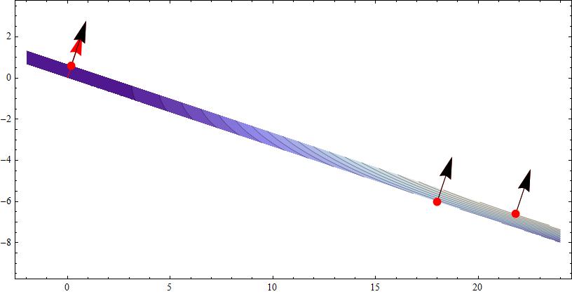
enter image source here

The qualification is left to the reader.

Note. Of course if the evaluation gives zero we will continue the qualification process but this is another chapter.