What is the order for the reaction 2"N"_2"O"_5(g) -> 4"NO"_2(g) + "O"_2(g)2N2O5(g)→4NO2(g)+O2(g)?
- What is the order of reaction?
- What is the concentration of
"O"_2O2 after 1010 minutes?
- What is
(Delta["NO"_2])/(Deltat)Δ[NO2]Δt ?
- What is the half-life of
"N"_2"O"_5N2O5 ?
- What is the concentration of
"N"_2"O"_5N2O5 after 100100 minutes?
- What is the order of reaction?
- What is the concentration of
"O"_2O2 after1010 minutes? - What is
(Delta["NO"_2])/(Deltat)Δ[NO2]Δt ? - What is the half-life of
"N"_2"O"_5N2O5 ? - What is the concentration of
"N"_2"O"_5N2O5 after100100 minutes?
2 Answers

Yes, graphing is the easiest way to do this (or this could be visually challenging!). In fact, learning how to use Excel is a very important skill. I've put a relatively short video on how to use Excel for chemistry here (which goes into graphs near the end):
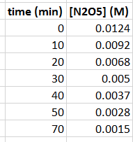
If you JUST put time in minutes on the
But with some trial and error...
-
graphing the second order integrated rate law does not work; while it does give a positive slope, the graph is curved (not linear), and thus is of the wrong order.
-
graphing the first order integrated rate law works to give a linear graph, confirming it is first order:
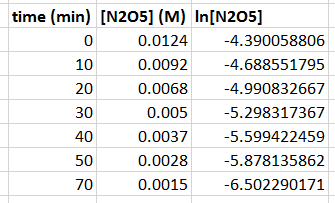
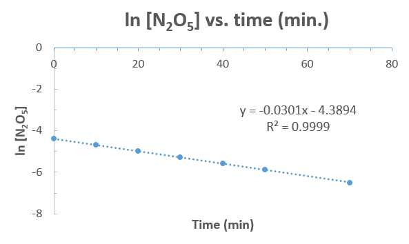
I've included the best fit line equation, which is given by:
bb(underbrace(overbrace(ln["N"_2"O"_5])^(y))_"ln of current conc." = underbrace(overbrace(-k)^(m))_"rate constant"overbrace(t)^(x) + underbrace(overbrace(ln["N"_2"O"_5]_0)^(b))_"ln of initial conc.")yln[N2O5]ln of current conc.=m−krate constantxt+bln[N2O5]0ln of initial conc. where
kk is the rate constant,["N"_2"O"_5][N2O5] is the concentration of"N"_2"O"_5N2O5 in"M"M , and[" "]_0[ ]0 means initial concentration. You know thattt means time in"min"min .
From looking at the best fit line equation, here is what you can immediately get from it:
"slope" = -kslope=−k
=> k = -"slope"⇒k=−slope
=> color(blue)(k = "0.0301 min"^(-1))⇒k=0.0301 min−1
"y-int." = -4.3894y-int.=−4.3894
=> color(blue)(["N"_2"O"_5]_0) = e^("y-int.") = e^(-4.3894) = color(blue)("0.0124 M")⇒[N2O5]0=ey-int.=e−4.3894=0.0124 M
And furthermore, the rate law for this would therefore be (from knowing what the order is):
r(t) = k["N"_2"O"_5]r(t)=k[N2O5]
This may or may not be a new concept, but let's consider something called an ICE Table (initial, change, equilibrium), which is normally a way to track the changes in concentration in a reaction on its way to "equilibrium", the point when the reaction has the same rate forwards and backwards.
In the ICE Table below, the coefficients in front of
2"N"_2"O"_5(g) -> 4"NO"_2(g) + "O"_2(g)2N2O5(g)→4NO2(g)+O2(g)
"I"" ""0.0124 M"" "" ""0 M"" "" "" ""0 M"I 0.0124 M 0 M 0 M
"C"" "-2x" "" "" "+4x" "" "" "+xC −2x +4x +x
"E"" ""0.0092 M"" "" "4x" "" "" "" "xE 0.0092 M 4x x
Well, we can track the progress of the reaction using the reaction quotient,
Since we know that the change in concentration of
And since
r(t) = k["N"_2"O"_5]r(t)=k[N2O5]
r(t) = 3.735 xx 10^(-4) "M/min" = |overbrace(-)^"consumption"1/2 overbrace((Delta["N"_2"O"_5])/(Deltat))^"Initial rate"|r(t)=3.735×10⁻⁴M/min=∣∣ ∣ ∣ ∣∣consumption−12Initial rateΔ[N2O5]Δt∣∣ ∣ ∣ ∣∣
= overbrace(+)^"production"1/4 overbrace((Delta["NO"_2])/(Deltat))^"Initial rate"=production+14Initial rateΔ[NO2]Δt
So, it is:
color(blue)((Delta["NO"_2])/(Deltat)) = 4/2 xx 3.735 xx 10^(-4) "M/min"Δ[NO2]Δt=42×3.735×10−4M/min
= color(blue)(7.47 xx 10^(-4) "M/min")=7.47×10−4M/min
ln["N"_2"O"_5] = -kt + ln["N"_2"O"_5]_0ln[N2O5]=−kt+ln[N2O5]0
First, plug in
ln(1/2["N"_2"O"_5]_0) = -kt_"1/2" + ln["N"_2"O"_5]_0ln(12[N2O5]0)=−kt1/2+ln[N2O5]0
Now use the property that
ln\frac(1/2cancel(["N"_2"O"_5]_0))(cancel(["N"_2"O"_5]_0)) = -kt_"1/2"ln12[N2O5]0[N2O5]0=−kt1/2
=> -ln2 = -kt_"1/2"⇒−ln2=−kt1/2
Thus, the first-order half-life is given by:
=> color(green)(t_"1/2" = (ln2)/k)⇒t1/2=ln2k
And now, we can get:
color(blue)(t_"1/2") = (ln2)/("0.0301 min"^(-1))t1/2=ln20.0301 min−1
== color(blue)("23.03 min")23.03 min
"100 mins passed"/"23.03 min half-life" ~~ 4.34100 mins passed23.03 min half-life≈4.34 half-lives passed.
Therefore, the initial concentration
This means the concentration after
color(blue)(["N"_2"O"_5]_("100 min.")) = "0.0124 M" xx 1/(2^(4.34)) ~~ color(blue)(6.11 xx 10^(-4) "M")[N2O5]100 min.=0.0124 M×124.34≈6.11×10⁻⁴M
(or

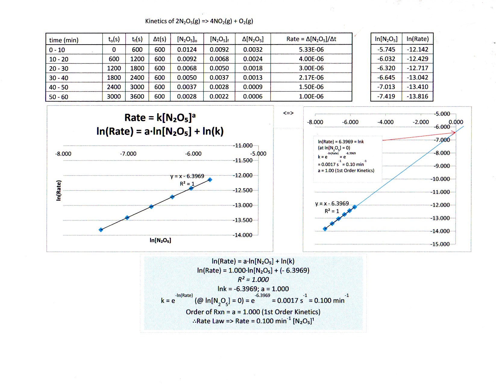
Kinetic Rate Law for Decomposition of
Explanation:
Kinetics of