How do you draw a phase diagram with a differential equation?
1 Answer

Well, it can be sketched by knowing data such as the following:
- normal boiling point (
#T_b# at#"1 atm"# ), if applicable - normal melting point (
#T_f# at#"1 atm"# ) - triple point (
#T_"tp", P_"tp"# ) - critical point (
#T_c,P_c# ) #DeltaH_"fus"# #DeltaH_"vap"# - Density of liquid & solid
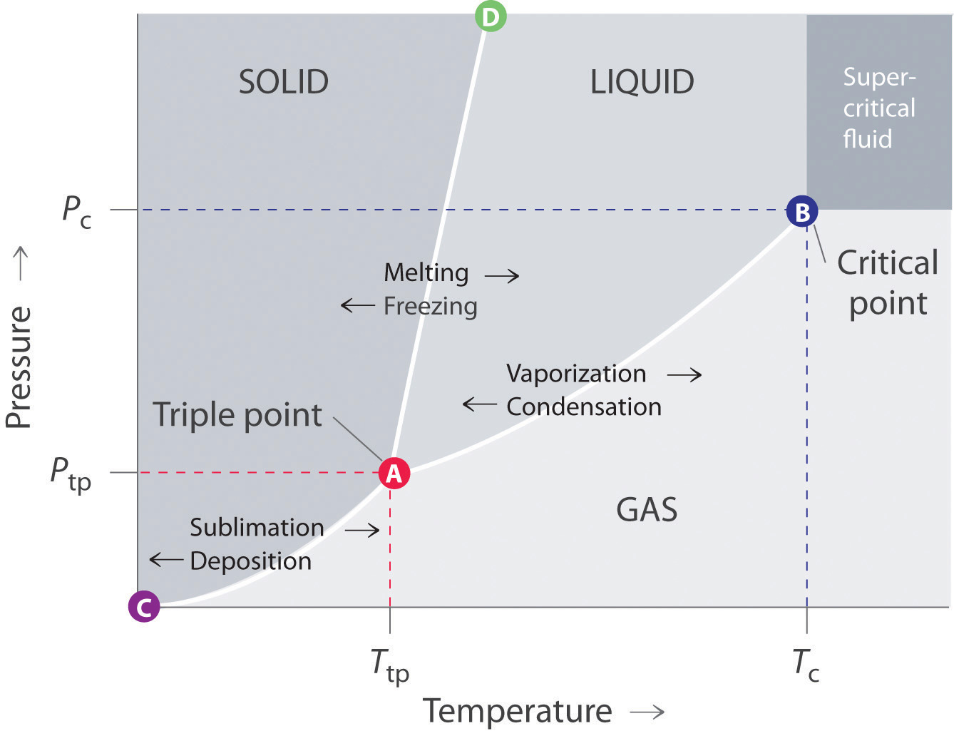
and by knowing where general phase regions are:
EXAMPLE DATA
Take
- sublimation temperature:
#"195 K"# (#-78.15^@ "C"# ) at#"1 atm"# - triple point:
#"216.58 K"# (#-56.57^@ "C"# ) at#"5.185 bar"# (#"5.117 atm"# ) - critical point:
#"304.23 K"# (#31.08^@ "C"# ) at#"73.825 bar"# (#"72.860 atm"# ) #DeltaH_"sub" = "25.2 kJ/mol"# at#"195 K"# (#-78.15^@ "C"# ) and#"1 atm"# - Density of liquid is greater than density of solid
#-># positive slope on the solid-liquid coexistence curve
DERIVING THE DIFFERENTIAL EQUATIONS
Next, consider the chemical potential
For example, suppose
#mu_((s)) = mu_((g))# , or#barG_((s)) = barG_((g))#
From the Maxwell Relation for the Gibbs' free energy, it follows that:
#dbarG_((g)) - dbarG_((s)) = dmu_((g)) - dmu_((s)) = dDeltamu_((s)->(g))#
#= -DeltabarS_"sub"dT + DeltabarV_"sub"dP = 0# where
#barS# and#barV# are the molar entropy and molar volume, respectively, of the phase change process, while#T# and#P# are temperature and pressure.
Therefore,
#DeltabarS_("sub")dT = DeltabarV_"sub"dP#
#=> (dP)/(dT) = (DeltabarS_"sub")/(DeltabarV_"sub")#
This gives the slope of the solid-gas coexistence curve. Obviously, the gas is less dense than the solid, so the slope will be positive.
Now, the
#DeltaG_"tr" = DeltaH_"tr" - T_"tr"DeltaS_"tr" = 0# ,
so
#DeltaS_"tr" = (DeltaH_"tr")/T_"tr"# .
Therefore, we obtain the Clapeyron differential equation:
#color(blue)((dP)/(dT) = (DeltabarH_"sub")/(T_"sub"DeltabarV_"sub"))#
And analogous equations can be derived for solid/liquid and liquid/vapor equilibria. The main difference is that for the liquid/vapor equilibrium, one can use the ideal gas law to rewrite it as:
#(dP)/(dT) = (DeltabarH_"vap")/(T_bDeltabarV_"vap") = (DeltabarH_"vap"P_"vap")/(T_b cdot RT_b)#
Therefore, for the liquid/vapor phase equilibrium, we have the Clausius-Clapeyron differential equation:
#1/P(dP)/(dT) = color(blue)((dlnP)/(dT) = (DeltabarH_"vap")/(RT_b^2))#
SOLVING THE DIFFERENTIAL EQUATIONS
This isn't that bad. In fact, all we are typically looking for is whether the slope is positive or negative, and often it is positive (except for water freezing).
Solid/Gas, Solid/Liquid Equilibria
#(dP)/(dT) = ((+))/((+)(+)) > 0#
This equation typically isn't evaluated formally, except in small temperature ranges where it is approximately linear.
But if we were to solve it, we would need an exceedingly small temperature range. Provided that is the case,
#int_(P_1)^(P_2) dP = int_(T_1)^(T_2) (DeltabarH_"tr")/(DeltabarV_"tr")1/T_"tr"dT#
In this small temperature range,
#color(blue)(DeltaP_"tr" ~~ (DeltabarH_"tr")/(DeltabarV_"tr")ln(T_(tr2)/T_(tr1)))#
Liquid/Vapor Equilibrium
#(dlnP)/(dT) = ((+))/((+)(+)^2) > 0#
This equation could be solved as a general chemistry exercise, but not in this form.
#int_(P_1)^(P_2) dlnP = int_(T_(b1))^(T_(b2))(DeltabarH_"vap")/R 1/T^2 dT#
Assuming a small-enough temperature range that
#color(blue)(ln(P_2/P_1) = -(DeltabarH_"vap")/R[1/T_(b2) - 1/T_(b1)])#
And this is the better-known form of the Clausius-Clapeyron equation from general chemistry. It is used to find boiling points at new pressures, or vapor pressures at new boiling points.
CONSTRUCTING THE PHASE DIAGRAM
The rest is using the data one could get from using these equations on one data point to get another data point.
I generally start by plotting the triple point and critical point, then outlining where the solid, liquid, and gas phase regions are. Then, I note which slopes are positive or negative, and sketch the curves from there.
- sublimation temperature:
#"195 K"# (#-78.15^@ "C"# ) at#"1 atm"# - triple point:
#"216.58 K"# (#-56.57^@ "C"# ) at#"5.185 bar"# (#"5.117 atm"# ) - critical point:
#"304.23 K"# (#31.08^@ "C"# ) at#"73.825 bar"# (#"72.860 atm"# )
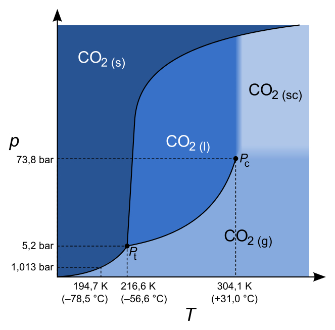
And as you can see, all the slopes here are positive as predicted.
