Question

Why is most-probable speed correspond to the top of the Maxwell-Boltzmann distribution curve, even though the root-mean-square speed is the highest? Why are average and root-mean-square to the right?

Answer 1

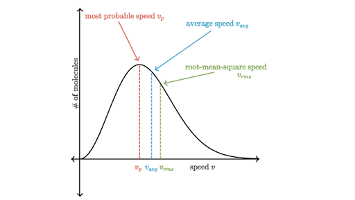
Because most-probable speed is most likely, i.e. a greater fraction of molecules will have that speed. It does NOT indicate that it is the highest in magnitude---only likelihood.

Let `upsilon_"mp"`, `<< upsilon >>`, and `upsilon_"rms"` be the most-probable, average, and root-mean-square speeds, respectively.

• `upsilon_"mp" = sqrt((2k_BT)/m)`
• `<< upsilon >> = sqrt((8k_BT)/(pim))`
• `upsilon_"rms" = sqrt((3k_BT)/m)`

From factoring out everything that is not `sqrt((k_BT)/m)`, you get the order `sqrt3 > 2sqrt(2/pi) > sqrt2`. That corresponds to the horizontal location of each type of speed on the graph. That is, `upsilon_"rms" > << upsilon >> > upsilon_"mp"`, since molecular speed increases from left to right on the x-axis.

The height on the y-axis does not indicate a faster speed.

I derive these equations below using the Maxwell-Boltzmann distribution (you would need to know how to perform derivatives, but the integrals used are tabled).

---

MOST PROBABLE SPEED

Given that `upsilon_"mp"` is the most-probable speed, then on the Maxwell-Boltzmann distribution plot, which is a probability density plot, it must be found at a local maximum, i.e. when the derivative `(df(upsilon))/(dupsilon)` of the speed distribution function `f(upsilon)` (with respect to speed `upsilon`) is `0`.

The `y` axis is the fraction of molecules with that speed, as the graph states, so it says that `upsilon_"mp"` is the speed that most molecules are likely to have (which is the intuitive interpretation of "most-probable" speed).

The Maxwell-Boltzmann speed distribution function (Physical Chemistry: A Molecular Approach, McQuarrie) is given as

`\mathbf(f(upsilon)dupsilon = 4pi(m/(2pik_BT))^"3/2" upsilon^2 e^(-m upsilon^2"/"2k_BT)dupsilon)`

where `k_B` is the Boltzmann constant, `T`is temperature, `m` is the mass of the gas, and `upsilon` is speed.

Taking the derivative with respect to `upsilon`, we would get:

`color(green)((df(upsilon))/(dupsilon))`

`= color(green)(4pi(m/(2pik_BT))^"3/2" d/(dupsilon)[upsilon^2e^(-m upsilon^2"/"2k_BT)])`

Using the product rule, we have `d/(dupsilon)[g(upsilon)h(k(upsilon))] = [g(upsilon)h'(k(upsilon))*k'(upsilon) + h(k(upsilon))g'(upsilon)]`, as follows:

`= 4pi(m/(2pik_BT))^"3/2" [upsilon^2cdot(-cancel(2)upsilon*m/(cancel(2)k_BT))e^(-m upsilon^2"/"2k_BT) + 2upsilone^(-m upsilon^2"/"2k_BT)]`

where `g(upsilon) = upsilon^2`, `h(upsilon) = e^(-m upsilon^2"/"2k_BT)`, and `k(upsilon) = -(m upsilon^2)/(2k_BT)`.

Now simply note that the constants can never be `0`, so they can be divided out to leave:

`= cancel(4pi(m/(2pik_BT))^"3/2") [e^(-m upsilon^2"/"2k_BT)(2upsilon - upsilon^3(m/(k_BT)))] = 0`

`= e^(-m upsilon^2"/"2k_BT)[2upsilon - upsilon^3(m/(k_BT))] = 0`

Of course, `e^x ne 0`, so the only thing that can be `0` is:

`0 = 2upsilon - upsilon^3(m/(k_BT))`

So we get, given that speeds are always positive:

`upsilon^(cancel(3)^(2)) (m/(k_BT)) = 2cancel(upsilon)`

`upsilon^2 = (2k_BT)/(m) => color(blue)(upsilon_"mp") = color(blue)(sqrt((2k_BT)/m))`

AVERAGE SPEED

The average speed can be gotten from the integral formula for averages, using the Maxwell-Boltzmann distribution from before:

`color(green)(<< upsilon >> = int_(0)^(oo) upsilonf(upsilon)dupsilon)`

`= 4pi(m/(2pik_BT))^"3/2" int_(0)^(oo) upsilon^3 e^(-m upsilon^2"/"2k_BT)`

Using this tabled integral:

`int_(0)^(oo) x^(2n+1)e^(-alphax^2)dx = (n!)/(2alpha^(n+1))`

we utilize `x = upsilon`, `n = 1`, and `alpha = m/(2k_BT)` to get:

`= 4pi(m/(2pik_BT))^"3/2" cdot 1/(2(m/(2k_BT))^(1+1))`

`= 4pi(m/(2pik_BT))^"3/2" cdot (2(k_BT)^2)/(m^2)`

`= 8pi(cancel(m)/(2pi))^"3/2"cancel((1/(k_BT))^"3/2") cdot ((k_BT)^(cancel("4/2")^"1/2"))/(m^(cancel("4/2")^"1/2"))`

`= 8pi(1/(2pi))^"2/2"cdot(1/(2pi))^"1/2" cdot ((k_BT)/(m))^"1/2"`

`= 4cdot ((k_BT)/(2pim))^"1/2"`

`=> color(blue)(<< upsilon >> = sqrt((8k_BT)/(pim)))`

ROOT-MEAN-SQUARE SPEED

Now, for the root-mean-square speed!

By definition, `upsilon_"rms" = sqrt(<< upsilon^2 >>)`. Back to the Maxwell-Boltzmann distribution! We update our previous formula for the average using the substitution `upsilon -> upsilon^2`:

`color(green)(<< upsilon^2 >> = int_(0)^(oo) upsilon^2f(upsilon)dupsilon)`

(You may want to compare this back to the average speed integral to see the difference.)

`= 4pi(m/(2pik_BT))^"3/2" int_(0)^(oo) upsilon^4 e^(-m upsilon^2"/"2k_BT)`

We use another tabled integral, since `2n+1 ne 4`:

`int_(0)^(oo) x^(2n)e^(-alphax^2)dx = (1cdot3cdot5cdots(2n-1))/(2^(n+1)alpha^n)(pi/(alpha))^"1/2"`

For this, `alpha = m/(2k_BT)`, `x = upsilon`, and `n = 2`.

`=> 4pi(m/(2pik_BT))^"3/2"[(1cdot(2*2-1))/(2^(2+1)(m/(2k_BT))^2)(pi/(m/(2k_BT)))^"1/2"]`

`= 4pi(m/(2pik_BT))^"3/2"[(3)/(8(m/(2k_BT))^2)(pi/(m/(2k_BT)))^"1/2"]`

`= 4pi(m/(2pik_BT))^cancel("3/2")[(3/8) * ((2k_BT)/m)^2cancel(((2pik_BT)/m)^"1/2")]`

`= 3/cancel(2)(cancel(pi)m)/(cancel(2)cancel(pi)k_BT) ((cancel(2)k_BT)/m)^2`

`= 3cancel((m)/(k_BT)) ((k_BT)/m)^cancel(2)`

`= (3k_BT)/m`

Therefore:

`color(blue)(upsilon_"rms") = sqrt(<< upsilon^2 >>) = color(blue)(sqrt((3k_BT)/m))`

NOW WHAT?

Now why the heck did we do all that? To get the comparable formulas, of course! We have:

• `upsilon_"mp" = sqrt((2k_BT)/m)`
• `<< upsilon >> = sqrt((8k_BT)/(pim))`
• `upsilon_"rms" = sqrt((3k_BT)/m)`

Notice that you can factor these out to get the following magnitude orders:

`sqrt3sqrt((k_BT)/m) > 2sqrt(2/pi)sqrt((k_BT)/(m)) > sqrt2*sqrt((k_BT)/m)`

That is, `color(blue)(upsilon_"rms" > << upsilon >> > upsilon_"mp")`

As your Maxwell-Boltzmann distribution plot shows, the root-mean square speed is farthest to the right on the graph, meaning that it is largest, and the most-probable speed is farthest to the left, meaning that it is smallest, as predicted in the comparison above.