Question

How do I find the eigenvalues for the finite potential well of width 2L?

Derive a transcendental equation for the allowed energies and solve it graphically in the finite well of the height `V_0`
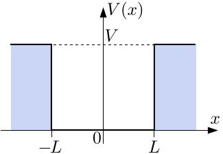
`V(x) = {(-V_0 ,|x|>=L),(0, "elsewhere"):}`

`alphatanalpha = k`(even parity)
`alphacotalpha = -k`(odd parity)

i hope that u understand what `alpha and k` are.

but to mark the energy eigenvalues

i had to make circle of radius `alpha + k`
what is the physical reason behind this?

Answer 1

Here is the Excel sheet I made while doing this.

The radius of the circle just tells you what you set the height of your potential well to be. However, its radius is given by `sqrt(alpha^2L^2 + k^2L^2)` in your notation...

`lim_(V_0 -> oo) "Finite Well" = "Infinite Potential Well"`

If we choose `V_0 = (20ℏ^2)/(2mL^2)` then we get three bound states in the well. These energy levels are shown below.

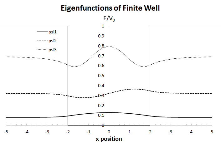
`ul(E" "" "" "" "" "" "E//V_0" "" "color(white)(.)"Quantum Number"" "" ")`
`(1.63948ℏ^2)/(2mL^2)" "" "0.081974" "" "1.28042`

`(6.44190ℏ^2)/(2mL^2)" "" "0.322095" "" "2.53809`

`(13.89150ℏ^2)/(2mL^2)" "color(white)(.)0.694575" "" "3.72713`

The graph below utilizes a well width of `2L = 4` as an example, with the appropriate coefficients `B`, `C`, and `D` to make the wave functions a practical scale.

---

Well, let's start by properly defining the problem... instead of defining a tunnelling problem with a barrier of width `2L`, which you have done, let's define a finite potential well of width `2L`...

`V(x) = {(V_0, |x| >= L), (0, -L < x < L):}`

That way, we get:

Then, let's define the eigenfunctions for each region `(I,II,III)`:

`psi_(I) = Ae^(-alphax) + Be^(alphax), " "" "" "" "-oo < x < -L`
`psi_(II) = Csin(kx) + Dcos(kx), " "-L < x < L`
`psi_(III) = Fe^(-alphax) + Ge^(alphax), " "" "" "" "L < x < oo`

where:

`alpha = sqrt((2m(V_0 - E))/ℏ^2)`, `" "E < V_0` for bound states
`k = sqrt((2mE)/ℏ^2)`

Since the wave function must vanish at `pmoo`, `A = 0` and `G = 0`. Furthermore, since the solution will have even and odd parity, we split the answer to the even and the odd solutions.

EVEN SOLUTIONS

For the even solutions, the `x = 0` line is a reflection axis, giving `B = F`. `cos` is even with respect to `x = 0`, so `C = 0` as well.

`psi_(I) = Be^(alphax), " "" "" "-oo < x < -L`
`psi_(II) = Dcos(kx), " "-L < x < L`
`psi_(III) = Be^(-alphax), " "" "" "L < x < oo`

Now we apply the continuity conditions.

`ul(psi_(I)(-L) = psi_(II)(-L))`:
`Be^(-alphaL) = Dcos(-kL)` `" "" "" "bb((1))`

`ul((dpsi_(I)(-L))/(dx) = (dpsi_(II)(-L))/(dx))`:
`alphaBe^(-alphaL) = -kDsin(-kL)` `" "bb((2))`

`ul(psi_(II)(L) = psi_(III)(L))`:
`Dcos(kL) = Be^(-alphaL)` `" "" "" "" "bb((3))`

`ul((dpsi_(II)(L))/(dx) = (dpsi_(III)(L))/(dx))`
`kDsin(kL) = alphaBe^(-alphaL)` `" "" "" "bb((4))`

Taking `((2))/((1))`, we get the so-called transcendental equation:

`color(green)(alpha = ktan(kL))`

Now, let `u = alphaL` and `v = kL`. Here we have specified the quantum number to be `v`.

From the definitions of `alpha` and `k`, we define

`u_0^2 -= u^2 + v^2 = alpha^2L^2 + k^2L^2`

`= (2mL^2(V_0 - E))/ℏ^2 + (2mL^2E)/ℏ^2 = (2mL^2V_0)/ℏ^2`

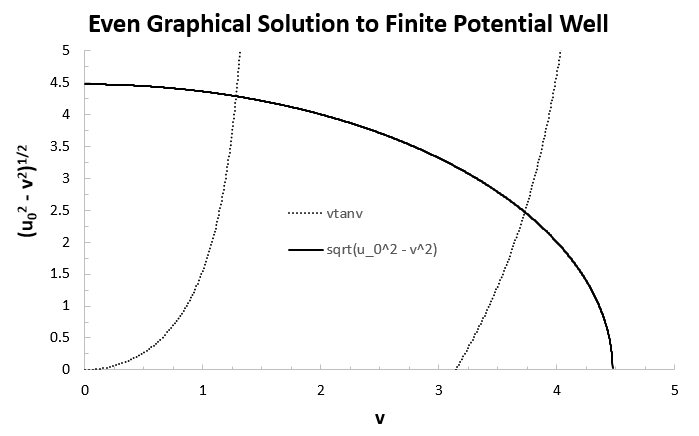
So now for the even solution, we can graph

`alphaL = kLtan(kL)`

or

`u = sqrt(u_0^2 - v^2) = vtanv`

Now we can simply use Excel to graph `sqrt(u_0^2 - v^2)` vs. `v` and `vtanv` vs. `v` on the same graph, and see where they intersect.

The intersections give the quantum numbers for each eigenvalue.

Suppose `V_0 = (20ℏ^2)/(2mL^2)`, so that `u_0^2 = 20`. Then we would get:

For the even solutions we got `v_1 ~~ 1.28042` and `v_3 ~~ 3.72713`. We'll see another one in the odd solutions later.

For now, each eigenvalue is given in terms of the quantum number `v_n`:

`v_n^2 = k_n^2L^2 = (2mL^2E_n)/ℏ^2`

`=> color(green)(E_n = (ℏ^2v_n^2)/(2mL^2))`

Now let's move on to the odd solutions.

ODD SOLUTIONS

Now the origin is a rotation axis, so that `B = -F` and `D = 0` instead. This gives new eigenfunctions:

`psi_(I) = Be^(alphax), " "" "" "-oo < x < -L`
`psi_(II) = Csin(kx), " "-L < x < L`
`psi_(III) = -Be^(-alphax), " "" "L < x < oo`

Now we apply the continuity conditions as before.

`ul(psi_(I)(-L) = psi_(II)(-L))`:
`Be^(-alphaL) = Csin(-kL)` `" "" "" "bb((1))`

`ul((dpsi_(I)(-L))/(dx) = (dpsi_(II)(-L))/(dx))`:
`alphaBe^(-alphaL) = kCcos(-kL)` `" "" "bb((2))`

`ul(psi_(II)(L) = psi_(III)(L))`:
`Csin(kL) = -Be^(-alphaL)` `" "" "" "bb((3))`

`ul((dpsi_(II)(L))/(dx) = (dpsi_(III)(L))/(dx))`
`kCcos(kL) = alphaBe^(-alphaL)` `" "" "" "bb((4))`

Taking `((2))/((1))` as before, we obtain the other transcendental equation:

`color(green)(alpha = -kcot(kL))`

Using the same substitutions as before, we again graph `sqrt(u_0^2 - v^2)` vs. `v` and `-vcotv` vs. `v` on the same graph and find the intersection(s) to get the quantum number(s).

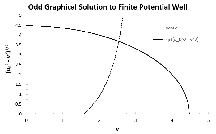
In this case our well only had three energy levels. Here we again had `u_0^2 = 20` and found one quantum number `v_2 ~~ 2.53809`.

COMBINED SOLUTIONS

And combining them onto one graph, we get the three energy levels in this finite well with `V_0 = (20ℏ^2)/(2mL^2)`:

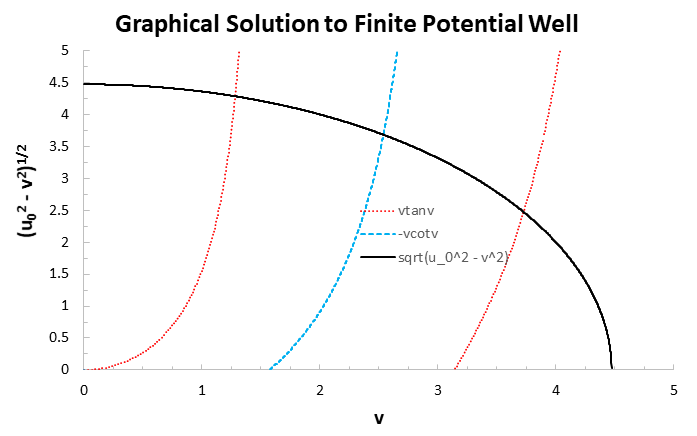
`color(blue)(E_1 = (1.63948ℏ^2)/(2mL^2))`

`color(blue)(E_2 = (6.44190ℏ^2)/(2mL^2))`

`color(blue)(E_3 = (13.89150ℏ^2)/(2mL^2))`

And of course, if we let `u_0 -> oo`, we recover the solutions to the infinite potential well. In that case the circular graph we have has a radius of `oo`.

The choice of `u_0^2` (and thus `V_0` in units of `ℏ^2/(2mL^2)`) just sets what the height of the potential well is.