Introduction to Parametric Equations
Key Questions
-
It depends on the curve you're analyzing,
In general, finding the parametric equations that describe a curve is not trivial. For the cases that the curve is a familiar shape (such as piecewise linear curve or a conic section) it's not that complicated to find such equations, due to our knowledge of their geometry.
As an example of a curve that's difficult to find the parametrization, just close your eyes and draw any curve on a piece of paper. Chances are that curve has a complicated description, and even if you found the equations describing it, it would probably be hard to work with them.
For problems that have these kind of difficulties, it's interesting to use numerical methods (such as piecewise linear approximations).An example that's not comprised of combinations of line segments or conic sections:
The cycloid is a curve with many interesting properties. Finding the parametric equations that describe it is very useful.
A cycloid is the curve generated by rotating a circle (of, say, radius
#a# ) over the#x# axis while tracing the path of the point initially at the origin.
The parameter adopted will be the angle described by the point intially at the origin, the center of the circle and the point of contact between the circle and the#x# axis.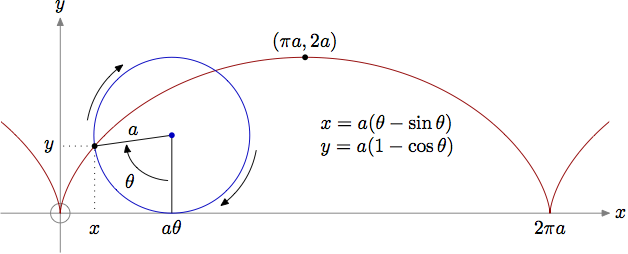
Basic geometry* will give us the equations:
#x(theta)=a[theta-sin(theta)]#
#y(theta)=a[1-cos(theta)]# *The
#x# coordinate is given by the difference between the arclenght#a theta# , wich is the distance between the origin and the projection over the#x# axis of the center of the circle, and the projection over the#x# axis of the radius of the circle associated with the tracing point, equal to#a sin(theta)# . The#y# coordinate is given by the difference between the height of the center of the circle, equal to the radius#a# , and the projection over the#y# axis of the radius of the circle associated with the tracing point, equal to#a cos(theta)# . Vinicius M. G. Silveira
·
1
·
Dec 16 2014
Vinicius M. G. Silveira
·
1
·
Dec 16 2014
-
The line segments between
#(x_0,y_0)# and#(x_1,y_1)# can be expressed as:
#x(t)=(1-t)x_0+tx_1#
#y(t)=(1-t)y_0+ty_1# ,
where#0 leq t leq 1# .The direction vector from
#(x_0,y_0)# to#(x_1,y_1)# is
#vec{v}=(x_1,y_1)-(x_0,y_0)=(x_1-x_0,y_1-y_0)# .
We can find any point#(x,y)# on the line segment by adding a scalar multiple of#vec{v}# to the point#(x_0,y_0)# . So, we have
#(x,y)=(x_0,y_0)+t(x_1-x_0,y_1-y_0)# ,
which simplifies to:
#(x,y)=((1-t)x_0+tx_1,(1-t)y_0+ty_1)# ,
where#0 leq t leq 1# .
Wataru
·
·
Sep 6 2014
-
Since we know that
#-1 le sint le 1# , the curve is limited to#-1 le x le 1# .By plugging
#x=sint# into#y=sin^2t# , we have#y=(sint)^2=x^2# .Hence, the curve is the portion of the parabola
#y=x^2# between#x=-1# and#x=1# , which looks like this: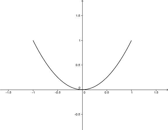
I hope that this was helpful.
Wataru
·
1
·
Oct 5 2014
-
Parametric equations are useful when a position of an object is described in terms of time
#t# . Let us look at a couple of example.Example 1 (2-D)
If a particle moves along a circular path of radius r centered at
#(x_0,y_0)# , then its position at time#t# can be described by parametric equations like:#{(x(t)=x_0+rcost),(y(t)=y_0+rsint):}# Example 2 (3-D)
If a particle rises along a spiral path of radius r centered along the
#z# -axis, then its position at time#t# can be described by parametric equations like:#{(x(t)=rcost),(y(t)=rsint),(z(t)=t):}# Parametric equations are useful in these examples since they allow us to describe each coordinate of the position of a particle separately in terms of time.
I hope that this was helpful.
Wataru
·
·
Oct 5 2014